
First Open-Coast HF Radar Observations of a 2-Phase Volcanic Tsunami, Tonga 2022
Codar Ocean Sensors, Mountain View, CA 94043, USA
*
Author to whom correspondence should be addressed.
Remote Sens. 2023, 15(9), 2325; https://doi.org/10.3390/rs15092325
Submission received: 4 March 2023
/
Revised: 13 April 2023
/
Accepted: 21 April 2023
/
Published: 28 April 2023
(This article belongs to the Special Issue HF Surface Wave Radar: Improving Performance and Extending Capabilities)
Abstract
:We describe results from coastal radar systems that observed anomalous current flows generated by the volcanic eruption in the Tongan archipelago on 15 January 2022 UTC, reporting the first radar detection of a volcanic tsunami. The eruption caused small tsunamis along the western U.S. Coast, generating some damage in a few harbors. The highest tsunami signal in U.S. tide gauge data from the California coast occurred at Arena Cove, with significant heights detected at Port San Luis and Crescent City. We analyze correlated wave orbital velocity detections by High Frequency (HF) radars along the coast between Gerstle Cove and Santa Barbara. Signals observed by the radars indicate that the event had two phases, each with its own distinct genesis: an initial weak surface disturbance, most likely generated by the wave of atmospheric pressure that moved outward from the blast source at just below the speed of sound, followed by a stronger disturbance that arrived approximately 3.5 h later, matching the arrival time for a wave moving entirely through the water from the volcano to the U.S. West Coast. We conclude that this phase consists of a conventional water wave tsunami and weaker waves generated by the pulse. We also report the detection of a small pulse-generated event off the west coast of Florida. Radar observations are compared with water level measurements at nearby tide gauges and a DART buoy, and with observations of barometric pressure. We point out that a Proudman near-resonance at the Tonga Trench is unlikely to explain the second phase observations. Comparison with tide gauge signals at San Francisco, generated by the Krakatoa eruption in 1883, support our conclusions.
1. Introduction
The submarine volcanic eruption that began on 20 December 2021 in the Tongan archipelago in the southern Pacific produced an unusual set of atmospheric and oceanic disturbances throughout the world. The eruption of the Hunga Tonga–Hunga Ha’apai (Tonga) volcano reached a large and powerful climax on 15 January 2022 UTC, which generated a large tsunami around local islands and moderate waves throughout the Pacific and other oceans. The event was unusual because of the complex explosive nature of the force field generating the tsunami, as opposed to an undersea earthquake. In addition to the sudden displacement of a large body of water, an atmospheric pressure pulse was generated that propagated world-wide. This pulse generated wave fields that arrived at many coasts much earlier than expected for earthquake-generated tsunamis. Tsunamis generated by atmospheric effects are well known and are typically called meteotsunamis [1]. This additional mechanism of wave generation complicates the interpretation of the oceanic disturbances recorded at many stations throughout the world. In this paper, we report the detection of unusual current flows seen off the California and West Florida coasts in locations equipped with coastal radar systems and compare the observations with those of nearby tide gauges. These radars are located on open coastlines and commonly obtainocean current information extending up to ~200 km offshore in arcs extending around the site. The measurements are therefore free of seiches (temporary disturbances in water level of a partially enclosed body of water) that often complicate tide gauge analyses [2]. The radar data is also of interest because wave propagation from Tonga to California is mostly through deep water, allowing simplified estimates of arrival times to be made. The Florida measurements involve propagation over a very wide, shallow continental shelf with land blocking the direct arrival of a conventional water wave generated tsunami. In the Pacific, we identify two phases of the current flows and conclude that both generation mechanisms were active. The results are found to be in fair agreement with data from nearby tide gauges and also consistent with Han and Yu’s analysis of tide gauge data from South America [3]. High-frequency radars in the eastern Tsugaru Strait, Japan, also observed the pulse-generated signals of the Tonga volcanic tsunami event [4].
In Section 2, we begin with some general discussion of the event and then briefly describe the radar ocean current measurement technique and its application to tsunami detection. In Section 3, we describe the radar observations and compare them with tide gauge and barometric observations. In Section 4, we compare observations of the 2022 Tonga tsunami with those of the 1883 Krakatoa eruption and the 2011 Japan tsunami and address the possibility of resonance effects at the Tonga Trench. The results are summarized in Section 5.
2. Materials and Methods
2.1. Tsunami Generation Mechanisms
The Tonga eruption and subsequent plume generated a broad range of atmospheric waves, some of which propagated around the world multiple times and were observed globally by various ground-based and space-borne instrumentation networks [5,6,7,8]. These included waves propagating at surface level and in the stratosphere and lower ionosphere. The most prominent pressure effect was a surface-guided Lamb wave, which was observed in barometric data propagating for four passages around the Earth over six days [5,9,10,11]. This data shows that the wave traveled at an average speed U of ~320 ± 5 m/s and that the wave form initially approximated a single pulse. For example, the outgoing signal from Tonga detected at Samoa [12] and Paso Robles, California [13] is characterized by a sharp positive pressure pulse, soon followed by a smaller negative pulse reminiscent of a soliton wave. When the pulse passes over large land masses, a more complex structure often develops.
It is well known that atmospheric effects can create meteotsunamis [1] that resemble a small earthquake-generated tsunami. Creating such a meteotsunami typically requires a sustained atmospheric disturbance with a substantial pressure change that moves at roughly the same speed as the underlying ocean waves, which can more easily happen in shallow waters. Lamb-wave generated tsunamis are relatively rare but were seen in the 1883 Krakatoa eruption [14]. This mechanism has led to them being termed volcanic meteotsunamis (VMTs) [1,15,16]. They can arrive much earlier than traditional tsunamis, indicating that the observed waves are generated as the pressure pulse approaches shorelines. In the present case, the pressure wave observed in California had an effective wavelength of ~500 km, with a somewhat longer positive half-cycle than negative [13]. This implies that the shallow water approximation is appropriate for water waves that would couple to the atmospheric wave. The corresponding phase velocity c(d) in water of depth d is given by:
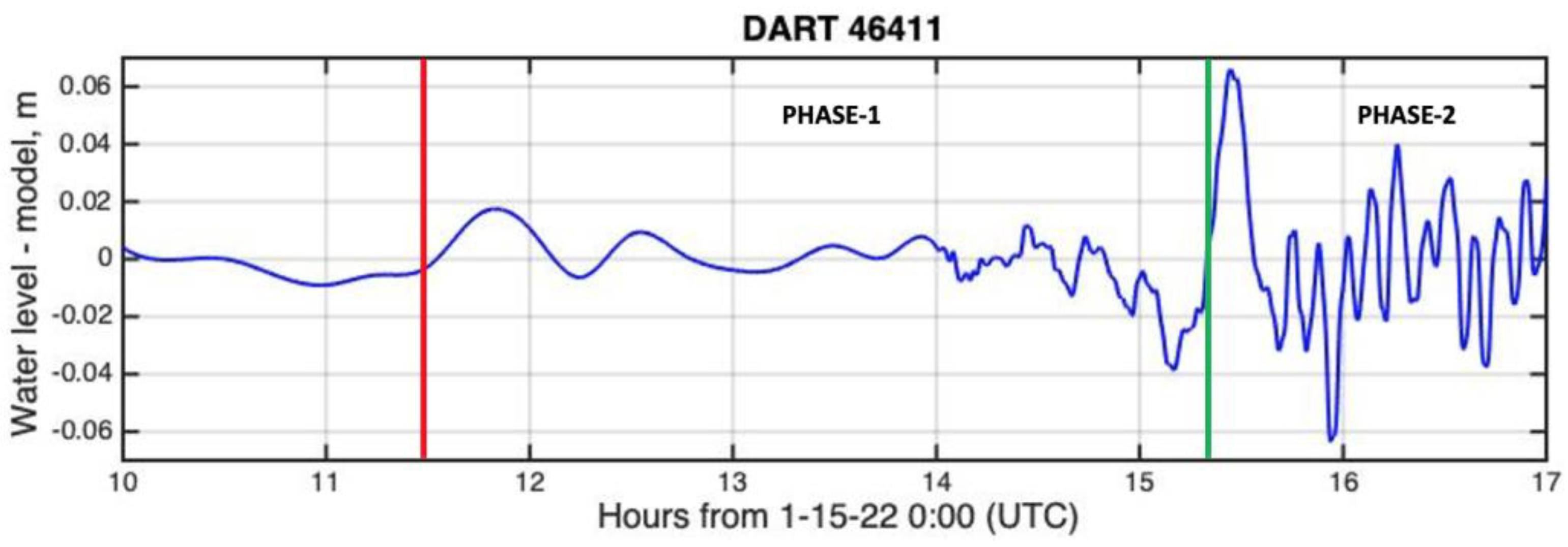
where g is the acceleration due to gravity. For the phase velocity to match the Lamb wave velocity, the required water depth is 10,400 m, which only occurs in very deep trenches. Thus, for most situations the VMT will lag behind the atmospheric pulse and become decoupled. However, the wave train will be continuously generated locally as the pulse moves across the water. An example of the resulting waveform from the Tonga tsunami can be seen in Figure 1, which shows detrended water level data from the DART buoy 46411 located off the coast of Northern California, where the water depth is approximately 4328 m [17]. The raw data was fitted with a spline function after tidal variations were removed, using a best-fit, 4th order polynomial over the 7 h of data shown in Figure 1. The estimated time of arrival of the pulse at the buoy is 11:30, 15 January 2022 UTC, which compares well with the start of the disturbance (see Figure 1) and well before a conventional tsunami could have arrived. When the wave phase velocity matches the pulse velocity, resonance occurs which amplifies the wave amplitude. The wave phase velocity at the buoy is ~206 m/s, which is well below the pulse velocity of 320 m/s required for resonance [18]. This implies that the signal is primarily generated by hydrostatic pressure changes. The passage of the pulse generated a damped wave train lasting at least 2 h. The peak-to-peak (pp) pressure pulse amplitude ΔP seen at Ukiah airport, California, the nearest site to the buoy which has 1 min time resolution, was ~2 mb [13]. The corresponding hydrostatic barometric sea level change h is related to the pressure increment as follows:
where ρ is the water density [4]. It follows that h ~2 cm, which is close to the value seen by the buoy. At ~14:00 UTC, the buoy automatically switched to high-speed data sampling. After 15:20 UTC, a stronger signal is seen with a higher frequency of oscillation. For clarity, we label these two segments of the data as phase-1 and phase-2.
h = ΔP/ρg
The second potential source of a tsunami wave is the abrupt water displacement due to the underwater volcano explosion and subsequent caldera collapse. Since the details of this generation mechanism are very uncertain due to the lack of instrumentation close to the site, it is difficult to even make rough estimates of the expected wave heights. From the reports of the waves seen in the Tonga archipelago, we can conclude that they were substantial, with waves of 12 to 15 m height reported at some islands [16]. For comparison, the pressure pulse amplitude recorded at Tonga, ~60 km from the volcanic source, was ~20 mb [5], which would create a hydrostatic VMT of ~0.2 m amplitude. Due to coastal shoaling, this wave could be amplified locally by a factor of ~4 before non-linear effects become important. These low values imply that most of the observed local wave motion was likely caused by some mechanism other than the pressure pulse. This was expected as soon as the extensive damage in the Tonga islands became known. The phase-2 signal characteristics shown in Figure 1 appear to indicate that it is due to a water-borne event in the Pacific basin, with the phase velocity obeying Equation (1). The estimated time of arrival of such a wave is ~16:00 UTC, close to the start of phase-2 behavior.
We note that the Tonga barometric record [5] is unusual in that the major initial pressure change is negative as opposed to positive in many other station records, e.g., as shown in Figure A3 of Appendix B. This has been attributed to differing velocities for positive and negative going pulses [19], but no physical model has yet been presented.
2.2. Radar Tsunami Detection
High frequency (HF) coastal radars have been used for the last 50 years to provide ocean observations. Their signals can propagate far beyond the horizon and are used mainly for providing area measurements of ocean surface current velocities and wave parameters. Crombie [20] first observed and identified the distinctive features of sea-echo in HF radar Doppler spectra. Barrick [21] derived expressions for the HF sea-echo Doppler spectrum in terms of the surface current velocities and the ocean wave directional spectrum. Methods were then developed [22,23] to interpret radar sea-echo spectra to give surface current velocity maps, directional ocean wave spectra and wind direction.
In 1979, Barrick first pointed out that HF radars could provide tsunami detection, as their orbital velocity is included in the current velocity field [24]. Following the 2011 Japan tsunami, algorithms were developed to detect the presence of a tsunami from radar-measured surface current velocities. The Japan tsunami signal was detected using offline analysis by 18 HF radars [25,26]. This was followed by the observation of weaker tsunamis and meteotsunamis [27,28].
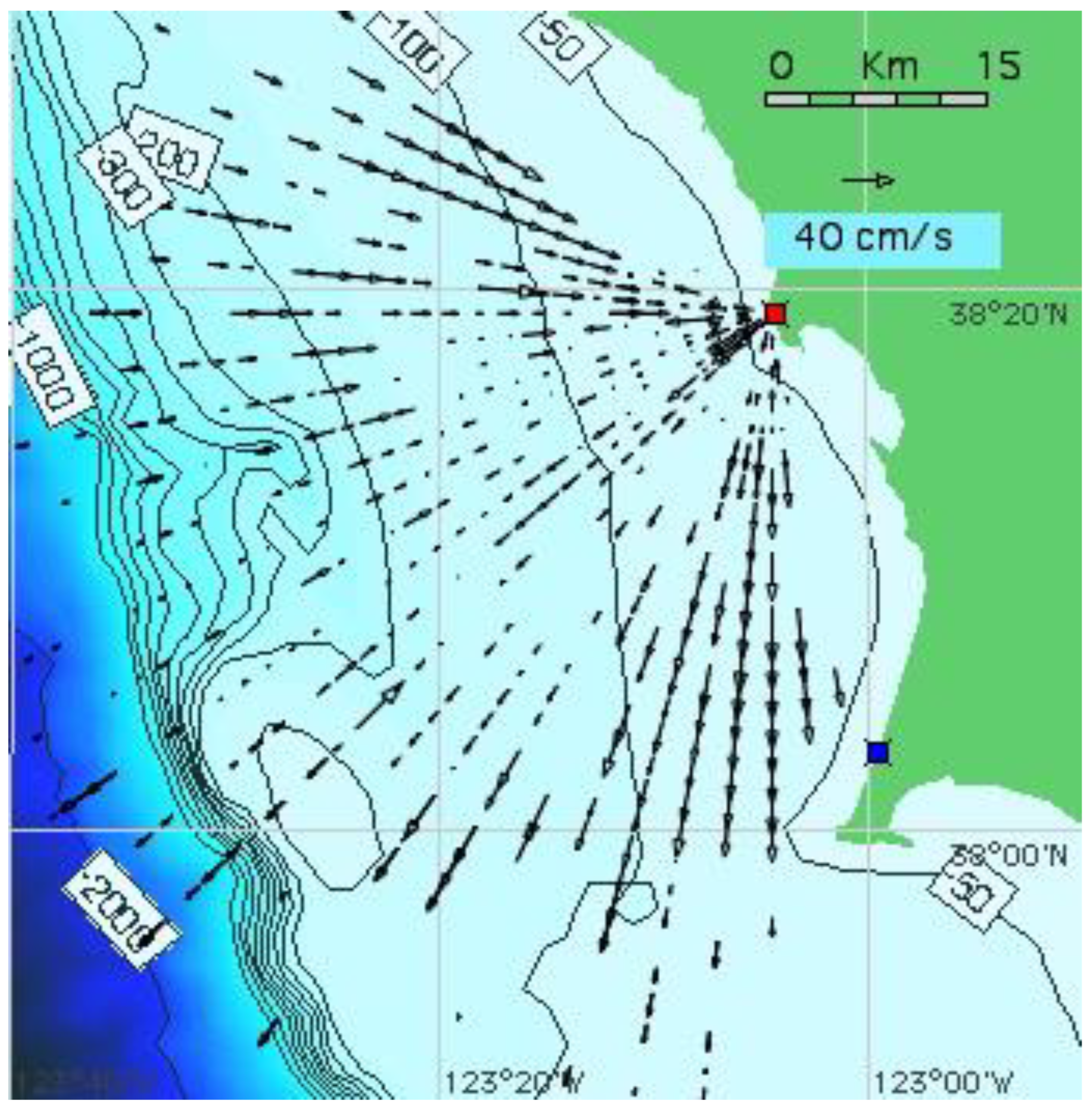
Tsunami detection capability is enhanced when shallow water extends far offshore and when the background current fields vary slowly. This capability added HF radar to existing methods used to detect tsunamis, e.g., the monitoring of seismic events [29], tide level changes, detection by buoys and coastal tide gauges and by using pressure recorders located on the ocean floor. At present, approximately 700 HF radar stations operate from many coastal locations, see for example https://codar.com (accessed on 28 February 2023), providing continuous measurement of surface current velocities and waves. Since the velocity fields extend far offshore, these radars can be used to provide local warnings of approaching tsunamis [25,26]. Radar tsunami detection is based on the analysis of the radial component of current velocities in the field of view. Figure 2 shows an example of radial current velocities measured with a radar located at Bodega Bay on the U.S. West Coast. For tsunami detection, the radar coverage area is divided into bands approximately 2 km wide and roughly parallel to the broad features of the depth contours. Radial current velocities are resolved parallel and perpendicular to the band boundaries and are then averaged over each band. We denote these averages, ‘band velocities’. A time series of perpendicular band velocities is then formed, which contains the characteristic orbital velocity oscillations produced by the tsunami. Two effects distinguish tsunami velocities from the background: (i) after arrival within the area monitored, there is strong correlation between velocities in neighboring bands and (ii) the oscillation period is much shorter than the diurnal tide cycle. At a given time, a quantity (known as the q-factor) is calculated which signals the tsunami arrival when it exceeds a pre-determined limit. We describe the algorithm briefly below; more details are given in [28].
The q-factor detection algorithm is essentially based on looking for correlations in band velocity changes that match the expected pattern for a tsunami approaching the radar site. The main steps in the algorithm are as follows:
- Within each band, if the velocity increment over two consecutive time intervals (typically 2 min each) has increased/decreased by an amount greater than a preset level, the q-factor for that band is incremented/decremented.
- If the maximum/minimum velocities for neighboring bands coincide within a preset value for consecutive time intervals, the q-factor level is further increased/decreased for those bands.
- Finally, if the velocity has increased/decreased over two consecutive time intervals for three adjacent area bands, the q-factor level is further incremented/decremented for those bands.
This process is repeated in real time for each radar averaging interval used to generate the radial current velocity maps.
Positive/negative q-factor values indicate that the orbital velocity of the tsunami is directed toward/away from the radar, indicating a rising or falling water level. To set the threshold defining the presence of a tsunami, an extended data set without tsunamis is analyzed to give residual q-factors to determine an optimal threshold value under normal conditions.
2.3. Radar Site Locations and Offshore Water Depths
In this subsection, we give the locations and offshore bathymetry characteristics of eight HF radars along the California Coast at Gerstle Cove (GCVE), Bodega Bay (BML1), Pt. Estero (ESTR), Diablo Canyon (DCSR), Port San Luis (LUIS), Point Sal (FBK1), Coal Oil Point (COP1), Summerland Sanitary District (SSD1) and one site on the Florida West Coast at Naples (NAPL). These are standard-range SeaSonde radars with compact crossed-loop antennas. Transmission frequencies are approximately 12 MHz and signal-to-noise ratios exceed 13 dB. The range resolution is about 2 km per range cell and the azimuthal resolution of the antenna pattern was measured to 1°. Results from these radars are compared with measurements from nearby NOAA tide gauges and a DART buoy. Coordinates of the radar sites are listed in Table 1.
Figure 3 shows the location of the radars, the Tonga volcano and DART 46411.
Radar and tide gauge locations and the offshore bathymetry are shown in Figure 4.
The location of DART buoy 46411 is 39°20′6″N 127°4′12″W, about 200 km west of Mendocino, Northern California [17].
2.4. The Effect of Water Depth on Tsunami Parameters
Tsunami orbital velocities are small in deep ocean basins, with values usually below the detectability threshold for HF radars. Typical tsunami periods are in the range 0.2 to 2 h. In the deep ocean, the tsunami wave amplitude is typically less than 1 m and wavelengths may be hundreds of kilometers. Tsunami orbital velocity and wave height increase when the wave moves onto the continental shelf. Orbital velocity increases rapidly with decreasing depth and can then exceed a detection threshold. Radar detection of a tsunami is therefore usually favored when shallow water extends far offshore. As the depth d decreases, the orbital velocity vo increases as defined by:
and the wave height h(d) increases according to:
where and are depths at two different locations [30]. The offshore bathymetry has a strong influence on coastal HF-radar tsunami detectability, which is highly site dependent. It can be studied in simulations to yield detectability thresholds. This has been done using numerical models for coastal tsunami propagation, based on the bathymetry offshore from the radar location. Our experience with tsunamis and site modeling [25,26,27,28,31] has led us to use the 200 m isobath as a convenient demarcation for likely radar detection of a tsunami wave with a run-up height of ~0.5 m, as observed by a nearby tide gauge. In most cases, this restricts the range of detection to ~20 km from the shore.
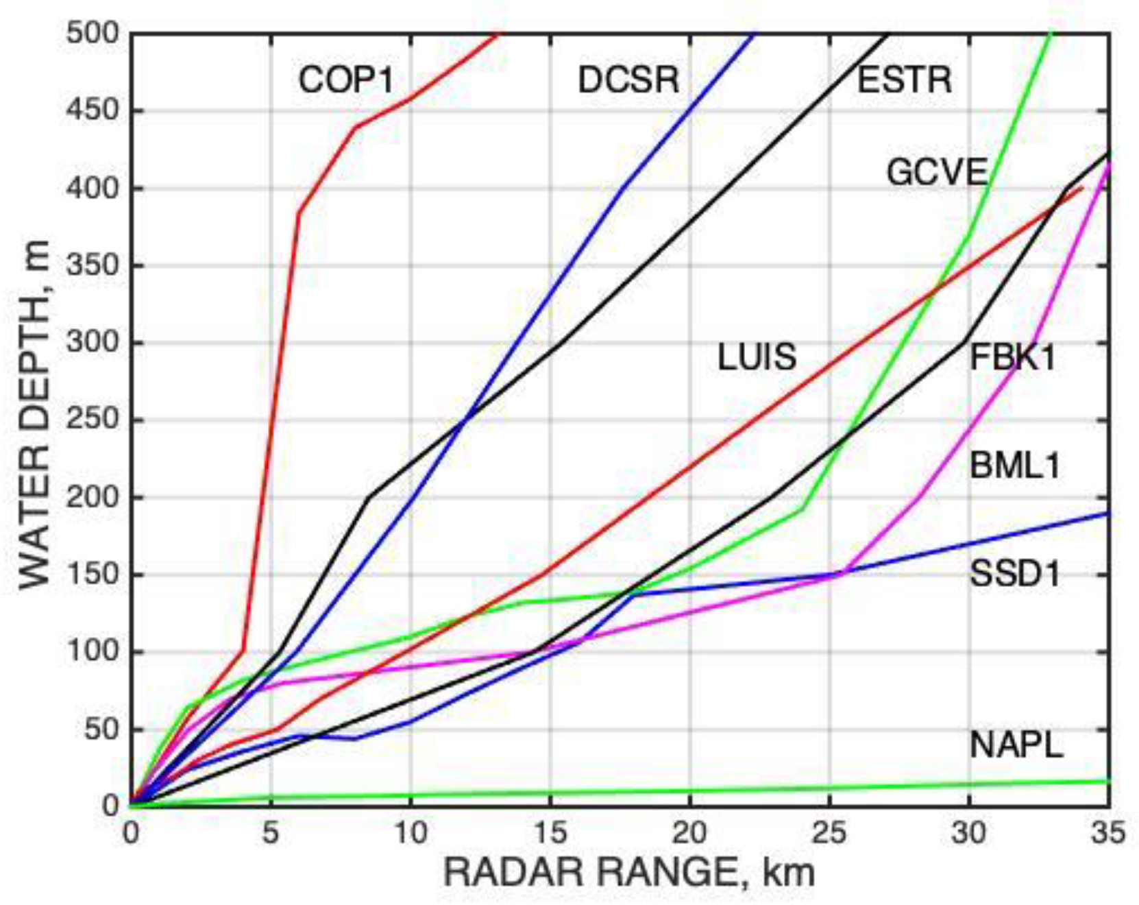
Figure 5 shows the depth vs. range for the nine radar sites studied in this paper. Depths were estimated from the NOAA Interactive Catalog [32] and the GEBCO 2020 Grid [33]. The water depths are interpolated spot values along the normal to the coast with grid resolutions of 0.5 to 5 km, depending on the bathymetry values shown on the charts. It follows from Figure 5 and Equation (3) that COP1 will have a lower tsunami detection capability than the other sites, as the water depth is greater close to shore, and that NAPL will have the highest tsunami detection capability.
3. Results
3.1. Radar Tsunami Detection on the U.S. West Coast and Florida: Band Velocities and q-Factors
We analyzed the radar data from the nine sites listed in Table 1 for three days following the Tonga event. These sites were selected primarily based on the wave heights reported on nearby tide gauges. Tsunami signals are clearly seen at eight of the sites, while the signal from COP1 is marginal, as expected, because of the deep water offshore.
A strong tsunami detection for both radar and tide gauge was obtained at LUIS. The radar band velocities and the corresponding q-factors are shown in Figure 6. The band velocities are overlaid to emphasize the correlations. In this plot, colors are plotted as follows: blue: band 2, red: band 3, green: band 4, black: band 5, maroon: band 6, cyan: band 7. Band 2 is 2–4 km offshore, other bands are incrementally 2 km further out.
A small perturbation can be seen at ~13.9 h, followed by a larger signal starting at ~16.6 h. Band-velocities and q-factors for the other sites with the strongest detection are given in Appendix A.
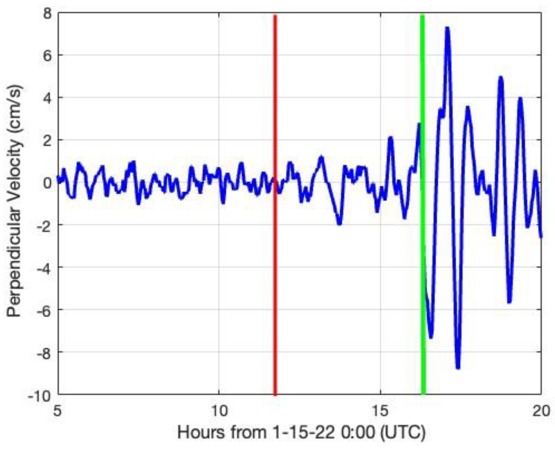
To get a clearer picture of the anomalous current flows detected by the LUIS radar, we averaged the measurements over bands 2–5 that are most sensitive to an incoming wave. This area averaging is expected to be useful in reducing the noise over the bands. The VMT signal is expected to be correlated over distances of >100 km, larger than the radar coverage area. The results are shown in Figure 7. The red line indicates the observed arrival time of the pressure pulse at Port San Luis and thus indicates the expected commencement of the phase-1 VMT. The green line indicates the expected arrival time of a conventional tsunami propagated entirely through the water. This time is based on an average velocity of 198 m/s for a long wavelength water wave propagating through deep water [8], corrected for the slowing occurring in shallow water due to subsea mountains and some islands close to the source, as quantified in Equation (1). Water-propagated waves travelling to the U.S. would be slowed and refracted while passing through this area.
After reaching the Tonga Trench [16], the tsunami encounters generally deep water all the way to the California coast, where it again slows due to the shallower water. This is expected to cause a delay of only a few minutes for the radar sites on the U.S. West Coast.
3.2. Tide Gauge Water Levels
The corresponding tide gauge data from Port San Luis is shown in Figure 8. This data shows the growth of a small signal starting at ~12 h UTC, indicating the start of the phase-1 event.
It is interesting that the onsets of the phase-2 event, marked by the sharp increase in both the orbital velocities and the water levels in Figure 7 and Figure 8, align quite well with the expected arrival time of a water-borne wave. This observation is supported by the data from the other radar sites in California, see Appendix A, and is discussed further in Section 3.4 below.
3.3. Barometric Pressure Observations
Figure 9 shows the detrended barometric pressure at the San Luis Obispo Airport [13] plotted vs. time, clearly showing the changes in pressure due to the arrival of the pulse at approximately 12 h UTC. The figure also shows subsequent small oscillations and higher amplitude oscillatory behavior occurring approximately 1.5 h after the main pulse arrival. Similar signals have been reported at other distant locations [9]. Barometric pressure observations from other sites close to the radars are shown in Appendix B. By tracking the strongest oscillatory pressure signal across much of the U.S. using airport barometric data, we have estimated that its velocity was 297 ± 30 m/s, which is close to that of the Lamb wave. These secondary disturbances may be a barometric signature of the smaller high-speed gravity waves reported by Wright et al. [34].
3.4. Tsunami Arrival Times
Table 2 summarizes the results for the expected and observed arrival times of the pressure pulse and the two phases of the volcanic tsunami. The observed pulse arrival times listed in column 4 are within 5 min of the expected values in column 3, consistent with a pulse velocity of 317 m/s [8] along the great circle routes indicated in the Figure 10 map, which is an azimuthal projection centered on Tonga obtained from the site ns6t.net at https://ns6t.net/azimuth/azimuth.html (accessed on 15 February 2023).
The observed phase-1 arrival times listed in column 5 of Table 2 show significant delays of up to 2 h, relative to the time of the pulse passage. This appears to be due to the amplification effect of the shallow coastal waters on the VMT orbital velocities for waves generated in deeper water that approach the radar sites, as determined by Equation (3). As noted in Section 2.1, the hydrostatic wave height caused by the pulse in deep water is only ~2 cm, with a correspondingly small orbital velocity. However, as a wave approaches shallow coastal waters, its phase velocity decreases, and both the wave height and orbital velocity increase, as described in Section 2.4. Thus, waves generated offshore can be amplified but also delayed as they approach the radar coverage area. This shoaling effect can lead to a growing signal after the pulse has passed. This feature is visible in Figure 7 and Figure 8.
The times of the abrupt increase of the signal oscillations marking the beginning of the phase-2 behavior are listed in Table 2 column 7 and are on the average within 11 min of the expected arrival times for a tsunami wave travelling from Tonga entirely through the water, listed in column 6. The expected times were calculated assuming that they were generated by the volcanic explosion on 15 January 2022 at 4:14:45 UTC [8] and traveled entirely through the water. The exact start time is unclear due to the lack of a quantitative generation mechanism. We used tsunami wave propagation modeling based on Equation (1) with an approximate averaged Pacific Ocean water depth of 4000 m along great circle paths. The estimates were corrected for the slowing in the shallow water due to subsea mountains and islands close to the source. They were also cross-checked against Port San Luis tide gauge readings for the 29 September 2009 Samoa earthquake-generated tsunami [35,36] that followed a similar path across the Pacific basin. The good agreement between Table 2 columns 6 and 7 strongly indicates that the phase-2 behavior is primarily due to abrupt water displacement generated near the volcano and is only weakly, if at all, due to the pulse mechanism. The suggested Lamb wave mechanism for the phase-2 behavior [19,37] provides no explanation for the agreement between the observations and predictions in Table 2.
Additional confirmation of the phase-2 mechanism is obtained from the observations at the NAPL site. The Tonga eruption generated many surface disturbances in other oceans, as well as the Pacific [8]. We report the radar detection of a small surface current disturbance off the west coast of Florida at Naples. The tide gauge on the Naples pier to the north of the radar detected a wave height of ~0.15 m pp approximately 40 min after the radar offshore detection and approximately 3.7 h after the pressure pulse had passed over the coast. By modeling the offshore water depth and calculating the corresponding wave position vs. time in the direction normal to the contours, we found that the wave and the pulse coincided approximately 330 km offshore, near the edge of the continental shelf. It appears that the pulse was able to generate a wave in the deeper water of the Gulf of Mexico, but the effect was reduced as the wave velocity decreased when the pulse entered shallower water. On the other hand, the wave already generated in deep water grew in amplitude according to Equation (3), when it crossed the continental shelf and thereafter propagated freely to the shore. We note that DART buoy 42409 in the Gulf of Mexico, with water depth at 3184 m, detected a sea level change of ~2.3 cm pp at 14:20 UTC on 15 January. This wave could grow to ~11.5 cm pp in 5 m deep water, close to the value seen at the Naples tide gauge. As expected, the detection at Naples confirms that the pressure pulse is the cause of the phase-1 event, as it is impossible for a conventional tsunami generated at Tonga to reach that location for at least another 14 h. Additionally, the absence of phase-2 behavior shows that it is not a deep water effect caused by the Lamb wave, at least in the Gulf of Mexico. This agrees with tide gauge observations [8] at many other locations outside the Pacific. Similar delayed effects are seen in the comparison of barometric and tide gauge data in the Atlantic, north of New York [35], where there is a broad continental shelf. In this case, the signals were driven by the pressure pulse returning to Tonga after passing through the antipodes. South of New York unsettled weather obscured the tide signals.
3.5. Tsunami Wave Height
The first-order analysis of tsunami wave motion applies in shallow water until nonlinear effects leading to waves breaking become significant [30]. This typically occurs when the water depth is only a few times the tsunami wave height. For the phase-2 observations discussed here, tsunami modeling indicates that nonlinearity becomes significant when the water depth is less than about 5 m. As tide gauges are usually located where water depth exceeds 5 m, first order tsunami modeling can be applied to radar-measured orbital velocities to predict the wave heights expected at nearby tide gauges.
One needs to be cautious in interpreting the tide gauge readings due to seiche effects [1] and wave reflections. Along the California Coast, tide gauges are located in protected inlets or harbors, so their readings may be dominated by local effects.
Table 3 shows very rough estimates of the phase-2 wave heights h(d) expected in 5 m deep water for the five radars with the strongest signals, along with readings from nearby tide gauges. The wave heights were derived from the orbital velocities and the water depths using Equations (3) and (4). There was no tide gauge close to FBK1; a rough estimate of wave height was made using data from the neighboring two gauges. The analysis was restricted to the first cycle of the orbital velocities and wave oscillations to minimize the impact of local effects. There is fair agreement except for comparisons at GCVE and LUIS that have higher tide gauge readings; possible explanations are as follows: the GCVE tide gauge is located approximately 40 km north of the radar, well outside the radar coverage area; the LUIS tide gauge is located within the San Luis Obispo Bay and is not directly exposed to the open ocean.
4. Discussion
It seems clear that the phase-1 signals are created by the atmospheric pressure pulse; to date, no other mechanism has been found to generate a precursor tsunami. However, this does not apply to the phase-2 tsunami, which is marked by an abrupt increase in the signal amplitude and a higher frequency of oscillation. Our analysis in Section 3.4 has shown that the arrival times of the phase-2 velocities are consistent with a long-wavelength water wave travelling from the volcano to the California Coast, with a shallow water velocity given by Equation (1). Lynett et al. [19] have shown that after the pulse has passed, multiple reflections from the shore can generate secondary wave trains lasting many hours. They conclude that, in the Pacific basin, the entire water disturbance can be attributed to the Lamb wave alone.
To test this hypothesis for tsunami waves travelling to California, we examined the records from the Krakatoa eruption in 1883 [38]. Choi et al. [39] have pointed out that, for California, the direct water wave from Krakatoa was blocked by Borneo and some Indonesian islands. The shortest alternative water path to California is via the Southern Ocean, south of New Zealand. A wave travelling this route would arrive ~20 h after the signature of the Lamb wave. The tide gauge data in San Francisco Bay for 2 days after the Krakatoa explosion is shown in [39]. Choi et al. also show a de-trended water level curve, which is reproduced in Figure 11a. The estimated arrival time of the Lamb wave is indicated by the red line. The estimated arrival time of the water wave is ~36 h GMT, which is marked by the green line. There is a slight increase in signal at that time [14,39], but it is statistically insignificant. Thus, it is reasonable to conclude that the 20 h record after ~16:00 GMT in Figure 11a is the signature of the Lamb wave. For comparison, we plot, in Figure 11b, the San Francisco Bay tide data for the Tonga event, which shows that the early phase-1 behavior for Tonga is similar to that for Krakatoa. It is also clear that there is no sharp increase in the Krakatoa signal strength after the phase-1 behavior has started, in contrast to the increased phase-2 behavior for Tonga. As the Tonga phase-2 signal starts at the expected arrival time of a water wave and is not seen in the overlapping Krakatoa data, it appears that it is mostly due to a water wave.
An important parameter in the comparison of Tonga with Krakatoa is the amplitude of the pressure pulse. Unfortunately, the quantitative data for the Krakatoa pressure pulse [38] is unavailable apart from Batavia gasometer pressure gauge readings, with an amplitude that exceeded 14 mb, the upper limit of the range of the gauge [38]. Another estimate can be made from the San Francisco tide data in Figure 11a. The maximum wave height of ~0.25 m pp is seen ~3 h after pulse arrival. This delay indicates that the wave originated far offshore in deep water. Working backwards using Equation (4) to correct for the shoaling effect on wave height), we estimate the corresponding wave height in 4000 m deep water to be ~5 cm pp. Since this wave could only be generated by the Krakatoa pressure pulse, this implies from Equation (2) that the hydrostatic barometric pressure signal was ~5 mb pp. For comparison, from Figure 9, we obtain the Tonga pressure pulse of 1.8 mb pp at the California coast, while measurements in Honolulu [13] give a slightly higher value of ~2.2 mb pp. From these estimates, we conclude that at San Francisco, the Lamb wave pressure pulse from Krakatoa was at least as big as that from Tonga and probably a factor of 2 larger.
We now address the possibility that the phase-2 disturbance was created by a Proudman resonance effect [19,40] during the passage of the pulse from the volcano to the California Coast. This phenomenon has been analyzed both analytically [40] and numerically [19,41,42] for meteotsunamis. As mentioned in Section 2.1, since the forcing term here is the rapidly moving Lamb wave, very deep water (~10,400 m) is required for the resonance condition, when the Froude number [34], defined by:
approximates unity. This occurs when the water-wave velocity c(d) matches that of the pressure pulse velocity U. In the present case, the Tonga Trench is the only location where this condition could be met. We estimate the Froude number in the trench to be >1.05 along the direct path from the volcano to California, i.e., slightly greater than the resonance condition.
The width of the trench when crossed by the California trajectory is about 47 km for 1.05 < < 1.18. From the duration of the pressure pulse seen at Samoa [12], we obtain an effective wavelength of the pulse of 860 km, which far exceeds the trench width. Assuming an optimistic case of = 1 for the full 47 km trench width, we use the results of a 2D numerical model with direct air pressure forcing [41] to estimate a wave height increase of <3% above the hydrostatic value of ~10 cm. It seems likely that the mismatch of the pulse wavelength to the trench width would reduce the magnitude of this effect. This implies that the phase-2 tsunami signal is unlikely due to Proudman resonance at the trench, a conclusion supported by the evidence of phase-2 behavior occurring at locations west of the volcano. For example, water-level signals seen on New Zealand DART buoys NZJ, NZK and NZL [6], where the water is relatively shallow between the volcano and the buoys, are similar to those seen by DART 46411, shown in Figure 1. This implies that the trench does not play a significant role in the generation of the phase-2 behavior, in agreement with the analysis of Han and Yu [3].
On the other hand, the modeling of Lynett et al. [19] and Harkrider and Press [18] shows that, even off-resonance, some amplification can occur. We conclude that the phase-2 behavior is most likely dominated by a direct water wave originating at the volcano combined with a smaller component from secondary scattering of the pulse generated waves. A rough estimate of the amplitude of this component can be obtained from the Krakatoa data in Figure 11, which shows a maximum wave height of ~20 cm pp. Since the Tonga pulse amplitude is probably less than half that of Krakatoa, we would expect the amplitude of this secondary component to be ~10 cm pp.
As a further demonstration of the two phases of the Tonga VMT, Figure 12 compares the Port San Luis tide gauge data for the Tonga volcanic event with that for the 2011 Japan and 2021 Alaska tsunamis, which were generated by earthquakes. For the 2011 and 2021 tsunamis, there was no visible phase-1 event, which is consistent with the absence of pressure pulses in the earthquake-generated tsunamis.
5. Conclusions
We have described the first radar observations of a 2-phase volcanic event. We conclude that the event most likely consisted of a small VMT, generated by the Tonga pressure pulse, and a following larger tsunami that was mainly generated near the Tonga eruption site and then travelled entirely through the water. A small component of this phase-2 event is likely to be pulse-generated secondary waves arriving from indirect paths to California. For the U.S. West Coast, this is at variance with the view that, in the Pacific, the phase-2 tsunami was generated by an atmospheric source, e.g., see [11,19], and in agreement with the views expressed in [3,8]. Our seiche-free areal radar observations are demonstrated to be reasonably consistent with the spot measurements from tide gauges and a DART buoy. Cases where tide gauge measurements are higher than the radar estimates may reflect local effects at the gauge sites. Radar and tide gauge measurements on the Florida West Coast are consistent with a pulse generated event only, as expected from the presence of a land barrier between the radar site and Tonga. We also provide a comparison of San Francisco Bay tide gauge data from the Krakatoa eruption with that from the Tonga event, which supports the conclusion that the phase-2 tsunami is primarily a water wave.
We plan to look for further U.S. East Coast tsunami radar detections from the Tonga eruption. These signals are of particular interest in their own right because there would be no water-propagated tsunami to complicate the observations. The broad continental shelf on the U.S. East Coast extends over the entire radar coverage area for ~20 installations, improving the detectability of the signal. Unfortunately, unsettled weather off the U.S. East Coast complicates the analysis of data from many of these sites.
Coastal radar systems can detect tsunami wave motions over a wide offshore area compared to the spot measurements of buoys or tide gauges. This can provide tsunami warnings localized to the area near the radar and a complementary two-dimensional view of the phenomenon. As more radar sites become established, improved analysis will be possible by combining data in areas of signal overlap.
Author Contributions
Conceptualization, B.L. and D.B.; methodology, B.L. and D.B.; software, B.L., M.L. and H.P.; validation, C.W., M.L. and H.P.; formal analysis, B.L.; investigation, B.L. and C.W.; resources, M.L. and H.P.; data curation, M.L. and H.P.; writing—original draft preparation, B.L.; writing—review and editing, B.L., C.W., M.L. and H.P. All authors have read and agreed to the published version of the manuscript.
Funding
This research received no external funding.
Data Availability Statement
Requests for data should be made to the lead author.
Acknowledgments
We are grateful to the individuals and institutions that maintain the radar systems and provided the data used in this paper: Deedee Shideler of Bodega Marine Laboratory, Ian Robbins of California Polytechnic State University, San Luis Obispo, CA, Hector Aguilar of Codar Ocean Sensors. Data from Bodega Bay and Gerstle Cove was provided by the University of California, Davis, Bodega Marine Laboratory. The west coast radar sites are supported by the Southern California Coastal Ocean Observing System and the Central and Northern California Coastal Ocean Observing System. These are both Regional Associations of NOAA’s Integrated Ocean Observing System (IOOS). NAPL site and data support was through University of South Florida’s (USF) College of Marine Science via the Coastal Ocean Monitoring and Prediction System program and by NOAA via the U.S. IOOS Office through the Southeast Coastal Ocean Observing Regional Association. USF HF Radar Network activity support from Clifford Merz is gratefully acknowledged.
Conflicts of Interest
The authors declare no conflict of interest.
Appendix A
In this Appendix, we show the band velocity and q-factor data for the radar sites listed in Table 1 with the strongest tsunami detection. Colors indicate the 2 km area bands used in the calculation, as described in the main text.
Figure A1.
Observations of the stronger phase-2 event for radar sites BML1, ESTR, LUIS, FBK1. (a) Band velocities. (b) Corresponding derived q-factors plotted vs. hours from 15 January 2022 0:00 UTC.
Figure A1.
Observations of the stronger phase-2 event for radar sites BML1, ESTR, LUIS, FBK1. (a) Band velocities. (b) Corresponding derived q-factors plotted vs. hours from 15 January 2022 0:00 UTC.

Figure A2.
Observations of the weaker phase-1 event at radar sites BML1, ESTR, LUIS, FBK1, California and NAPL at Naples, Florida. (a) Band velocities. (b) Derived q-factors plotted vs. hours from 15 January 2022 0:00 UTC. Note the different axis scales used for Naples.
Figure A2.
Observations of the weaker phase-1 event at radar sites BML1, ESTR, LUIS, FBK1, California and NAPL at Naples, Florida. (a) Band velocities. (b) Derived q-factors plotted vs. hours from 15 January 2022 0:00 UTC. Note the different axis scales used for Naples.

Appendix B
In this Appendix, we show the barometric pressure data from tide gauge sites close to the radars. Data with 6 min time resolution is shown for Arena Cove, Point Reyes and Naples, obtained from the NOAA tide gauge web site [35], and with 1 min resolution for Port San Luis and Santa Barbara that have nearby airports [13].
Figure A3.
Pressure deviations from barometric data at Arena Cove, Point Reyes, Port San Luis, Santa Barbara, California and at Naples, Florida plotted vs. hours from 15 January 2022 0:00 UTC. Note the different axis scales used for Naples.
Figure A3.
Pressure deviations from barometric data at Arena Cove, Point Reyes, Port San Luis, Santa Barbara, California and at Naples, Florida plotted vs. hours from 15 January 2022 0:00 UTC. Note the different axis scales used for Naples.

References
- Rabinovich, A.B. Twenty-Seven Years of Progress in the Science of Meteorological Tsunamis Following the 1992 Daytona Beach Event. Pure Appl. Geophys. 2020, 177, 1193–1230. [Google Scholar] [CrossRef]
- Rabinovich, A.B. Seiches and harbor oscillations. In Handbook of Coastal and Ocean Engineering; Kim, Y.C., Ed.; World Scientific Publ.: Singapore, 2009; Chapter 9; pp. 193–236. [Google Scholar]
- Han, P.; Yu, X. An unconventional tsunami: 2022 Tonga event. Phys. Fluids 2022, 34, 116607. [Google Scholar] [CrossRef]
- Wang, Y.; Imai, K.; Mulia, I.E.; Ariyoshi, K.; Takahashi, N.; Sasaki, K.; Kaneko, H.; Abe, H.; Sato, Y. Data Assimilation Using High-Frequency Radar for Tsunami Early Warning: A Case Study of the 2022 Tonga Volcanic Tsunami. J. Geophys. Res. Solid Earth 2023, 128, e2022JB025153. [Google Scholar] [CrossRef]
- Wright, C.J.; Hindley, N.P.; Alexander, M.J.; Barlow, M.; Hoffmann, L.; Mitchell, C.N.; Prata, F.; Bouillon, M.; Carstens, J.; Clerbaux, C.; et al. Surface-to-space atmospheric waves from Hunga Tonga-Hunga Ha’apai eruption. Nature 2022, 609, 741–746. [Google Scholar] [CrossRef] [PubMed]
- Gusman, A.R.; Roger, J. Hunga Tonga-Hunga Ha’apai Volcano-Induced Sea Level Oscillations and Tsunami Simulations. GNS Science Webpage. 2022. Available online: https://www.gns.cri.nz/Home/Our-Science/Natural-Hazards-and-Risks/Tsunami/2022-Hunga-Tonga-Tsunami (accessed on 3 August 2022).
- Hunga Tonga Hunga-Ha’apai Volcano-Generated Tsunami, 15 January 2022 UTC. Main Event Page. Available online: https://nctr.pmel.noaa.gov/tonga20220115/ (accessed on 3 August 2022).
- Carvajal, M.; Sepúlveda, I.; Gubler, A.; Garreaud, R. Worldwide Signature of the 2022 Tonga Volcanic Tsunami. Geophys. Res. Lett. 2022, 49, e2022GL098153. [Google Scholar] [CrossRef]
- Harrison, G. Pressure anomalies from the January 2022 Hunga Tonga-Hunga Ha’apai eruption. Weather 2022, 77, 87–90. [Google Scholar] [CrossRef]
- Matoza, R.S.; Fee, D.; Assink, J.D.; Iezzi, A.M.; Green, D.N.; Kim, K.; Toney, L.; Lecocq, T.; Krishnamoorthy, S.; Lalande, J.M.; et al. Atmospheric waves and global seismo-acoustic observations of the January 2022 Hunga eruption, Tonga. Science 2022, 277, 6601. [Google Scholar] [CrossRef]
- Omira, R.; Ramalho, R.S.; Kim, J.; González, P.J.; Kadri, U.; Miranda, J.M.; Carrilho, F.; Baptista, M.A. Global Tonga tsunami explained by a fast-moving atmospheric source. Nature 2022, 609, 734–740. [Google Scholar] [CrossRef]
- Prata, F.; AIRES Pty Ltd. Available online: https://zenodo.org/record/6575810#.YuMEg_HMKZ0https:%2F%2Fzenodo.org%2Frecord%2F6575810%2Ffiles%2Famerican_samoa.png%3Fdownload=1 (accessed on 10 November 2022).
- Iowa State University, Environmental Mesonet. Available online: https://mesonet.agron.iastate.edu/request/asos/1min.phtml#://doi.org/10.1186/s40562-022-00232-z (accessed on 10 November 2022).
- Ewings, M.; Press, F. Tide Gauge Disturbances from the Great Eruption of KRAKATOA; Tech. Report on Seismology No. 27; Columbia University: New York, NY, USA, 1953. [Google Scholar]
- Lowe, D.J.; De Lange, W.P. Volcano-meteorological tsunamis, the c. AD 200 Taupo eruption (New Zealand) and the possibility of a global tsunami. Holocene 2000, 10, 401–407. [Google Scholar] [CrossRef]
- Terry, J.; Goff, J.; Winspear, N.; Bongolan, V.; Fisher, S. Tonga volcanic eruption and tsunami, January 2022: Globally the most significant opportunity to observe an explosive and tsunamigenic submarine eruption since AD 1883 Krakatau. Geosci. Lett. 2022, 9, 24. [Google Scholar] [CrossRef]
- DART® (Deep-Ocean Assessment and Reporting of Tsunamis). Available online: https://nctr.pmel.noaa.gov/Dart/ (accessed on 20 September 2022).
- Harkrider, D.; Press, F. The Krakatoa air-sea waves: An example of pulse propagation in coupled systems. Geophys. J. R. Astron. Soc. 1967, 13, 149–158. [Google Scholar] [CrossRef]
- Lynett, P.; McCann, M.; Zhou, Z.; Renteria, W.; Borrero, J.; Greer, D.; Cinar, G.E. Diverse tsunamigenesis triggered by the Hunga Tonga-Hunga Ha’apai eruption. Nature 2022, 609, 728. [Google Scholar] [CrossRef] [PubMed]
- Crombie, D.D. Doppler spectrum of sea echo at 13.56 MHz. Nature 1955, 75, 681–682. [Google Scholar] [CrossRef]
- Barrick, D.B. First-order theory and analysis of MF/HF/VHF scatter from the Sea. IEEE Trans. Antenna Propag. 1972, AP-20, 2–10. [Google Scholar] [CrossRef]
- Lipa, B.; Nyden, B.; Ullman, B.D.; Terrill, E. SeaSonde Radial Velocities: Derivation and Internal Consistency. IEEE J. Ocean. Eng. 2006, 31, 850–861. [Google Scholar] [CrossRef]
- Lipa, B.J.; Barrick, D.E. Least-squares methods for the extraction of surface currents from CODAR crossed-loop data: Application at ARSLOE. IEEE J. Ocean. Eng. 2006, OE-8, 226–253. [Google Scholar] [CrossRef]
- Barrick, D.E. A coastal radar system for tsunami warning. Remote Sens. Environ. 1979, 8, 353–358. [Google Scholar] [CrossRef]
- Lipa, B.; Isaacson, J.; Nyden, B.; Barrick, D. Tsunami arrival detection with high frequency (HF) radar. Remote Sens. 2012, 4, 1448–1461. [Google Scholar] [CrossRef]
- Dzvonkovskaya, A. Ocean surface current measurements using HF radar during the 2011 Japan tsunami hitting Chilean coast. In Proceedings of the 2012 IEEE International Geoscience and Remote Sensing Symposium 2012, Munich, Germany, 22–27 July 2012; pp. 7605–7608. [Google Scholar]
- Lipa, B.; Barrick, D.; Diposaptono, S.; Isaacson, J.; Jena, B.K.; Nyden, B.; Rajesh, K.; Kumar, T.S. High Frequency (HF) Radar detection of the weak 2012 Indonesian tsunamis. Remote Sens. 2012, 4, 2944–2956. [Google Scholar] [CrossRef]
- Lipa, B.; Parikh, H.; Barrick, D.; Roarty, H.; Glenn, S. High Frequency Radar Observations of the June 2013 US East Coast Meteotsunami. Nat. Hazards. 2014, 74, 109–122. [Google Scholar] [CrossRef]
- Poli, P.; Shapiro, N.M. Rapid characterization of large volcanic eruptions: Measuring the impulse of the Hunga Tonga explosion from teleseismic waves. Geophys. Res. Lett. 2022, 49, 8. [Google Scholar] [CrossRef]
- Lipa, B.; Barrick, D.; Bourg, J.; Nyden, B. HF radar detection of tsunamis. J. Oceanogr. 2006, 2, 705–716. [Google Scholar] [CrossRef]
- Lipa, B.; Barrick, D.; Isaacson, J. Coastal Tsunami Warning with Deployed HF Radar Systems. In Tsunami; Mokhtari, M., Ed.; InTech: London, UK, 2016; Available online: http://www.intechopen.com/books/tsunami/coastal-tsunami-warning-with-deployed-hf-radar-systems (accessed on 15 November 2022). [CrossRef]
- Office of Coast Survey. Available online: https://www.charts.noaa.gov/InteractiveCatalog/nrnc.shtml (accessed on 20 April 2023).
- GEBCO Compilation Group. GEBCO 2021 Grid; NERC EDS British Oceanographic Data Centre NOC: Liverpool, UK, 2021. [Google Scholar] [CrossRef]
- Wright, C.; Hindley, N.; Alexander, M.J.; Barlow, M.; Hoffmann, L.; Mitchell, C.; Yue, J. Tonga eruption triggered waves propagating globally from surface to edge of space. Nature 2022, 609, 741–746. [Google Scholar] [CrossRef] [PubMed]
- Tide Gauge Water Levels. Available online: https://tidesandcurrents.noaa.gov/waterlevels.html?id=9412110 (accessed on 25 September 2022).
- Available online: https://en.wikipedia.org/wiki/2009_Samoa_earthquake_and_tsunami (accessed on 20 April 2023).
- Williams, D.A.; Horsburgh, K.J.; Schultz, D.M.; Hughes, C.W. Proudman Resonances with tides, bathymetry and variable atmospheric forcings. Nat. Hazards 2021, 106, 1169–1194. [Google Scholar] [CrossRef]
- Symons, G.J. (Ed.) The Eruption of Krakatoa and Subsequent Phenomena; Report to Royal Society; 1888; Available online: https://hdl.handle.net/2027/hvd.32044032825895 (accessed on 26 November 2022).
- Choi, B.H.; Pelinovsky, E.; Kim, K.O.; Lee, J.S. Simulation of the trans-oceanic tsunami propagation due to the 1883 Krakatau Volcanic eruption. Nat. Hazards Earth Syst. Sci. 2003, 3, 321. [Google Scholar] [CrossRef]
- Proudman, J. The effects on the sea of changes in atmospheric pressure. Geophys. Suppl. Mon. Not. R. Astron. Soc. 1929, 2, 197–209. [Google Scholar] [CrossRef]
- Vilibic, I. Numerical simulations of the Proudman resonance. Cont. Shelf Res. 2008, 28, 574–581. [Google Scholar] [CrossRef]
- Amores, A.; Monserrat, S.; Marcos, M.; Argüeso, D.; Villalonga, J.; Jordà, G.; Gomis, D. Numerical simulation of atmospheric Lamb waves generated by the 2022 Hunga-Tonga volcanic eruption. Geophys. Res. Lett. 2022, 49, e2022GL098240. [Google Scholar] [CrossRef]
Figure 1.
DART water level fluctuations plotted vs. hours from 15 January 2022 00:00 UTC, showing behavior shortly after passage of the Lamb wave at ~11.5 h UTC. Phase-1 and phase-2 start times are indicated by the red and green lines.
Figure 1.
DART water level fluctuations plotted vs. hours from 15 January 2022 00:00 UTC, showing behavior shortly after passage of the Lamb wave at ~11.5 h UTC. Phase-1 and phase-2 start times are indicated by the red and green lines.

Figure 2.
An example of a radial current map measured by a radar located at Bodega Bay, California. Contours are labeled with the depth in meters. The arrow at the upper right indicates the current velocity scale.
Figure 2.
An example of a radial current map measured by a radar located at Bodega Bay, California. Contours are labeled with the depth in meters. The arrow at the upper right indicates the current velocity scale.

Figure 3.
The location of the Hunga Tonga-Hunga Ha’apai submarine volcano in the Tongan archipelago, radar sites that detected the tsunami located in California and Florida and DART buoy 46411. For reference, the distance between Tonga and Los Angeles is ~8500 km.
Figure 3.
The location of the Hunga Tonga-Hunga Ha’apai submarine volcano in the Tongan archipelago, radar sites that detected the tsunami located in California and Florida and DART buoy 46411. For reference, the distance between Tonga and Los Angeles is ~8500 km.

Figure 4.
Locations of radar sites (red), tide gauges (yellow): (a) Northern California, (b) Southern California, (c) Florida West Coast. Depth contours are every 100 m in (a) and (b), and every 4 m in (c).
Figure 4.
Locations of radar sites (red), tide gauges (yellow): (a) Northern California, (b) Southern California, (c) Florida West Coast. Depth contours are every 100 m in (a) and (b), and every 4 m in (c).

Figure 5.
Water depth plotted as a function of range normal to the coast for the radar sites listed in Table 1.
Figure 5.
Water depth plotted as a function of range normal to the coast for the radar sites listed in Table 1.

Figure 6.
Tsunami detection at LUIS on 15 January 2022 UTC. (Left) band velocities; (right) derived detection q-factors. See text for the color coding.
Figure 6.
Tsunami detection at LUIS on 15 January 2022 UTC. (Left) band velocities; (right) derived detection q-factors. See text for the color coding.

Figure 7.
Averaged LUIS orbital velocities from bands 2–5 plotted vs. time. The observed arrival time of the pressure wave and the estimated arrival time of a conventional tsunami are indicated by the vertical red and green lines.
Figure 7.
Averaged LUIS orbital velocities from bands 2–5 plotted vs. time. The observed arrival time of the pressure wave and the estimated arrival time of a conventional tsunami are indicated by the vertical red and green lines.

Figure 8.
Port San Luis water level data with tide model values subtracted, plotted vs. hours from 15 January 2022 0:00 UTC. Phase-1 and phase-2 start times are indicated by the red and green lines.
Figure 8.
Port San Luis water level data with tide model values subtracted, plotted vs. hours from 15 January 2022 0:00 UTC. Phase-1 and phase-2 start times are indicated by the red and green lines.

Figure 9.
Pressure deviations from a 5th order polynomial fitted to 24 h of data from San Luis Obispo Airport, California, plotted vs. hours from 15 January 2022 0:00 UTC.
Figure 9.
Pressure deviations from a 5th order polynomial fitted to 24 h of data from San Luis Obispo Airport, California, plotted vs. hours from 15 January 2022 0:00 UTC.

Figure 10.
Azimuthal projection showing in blue a simulated pressure pulse from the Tonga volcano arriving at the U.S. West Coast, great circle paths from Tonga, circles centered on Tonga and latitude and longitude values.
Figure 10.
Azimuthal projection showing in blue a simulated pressure pulse from the Tonga volcano arriving at the U.S. West Coast, great circle paths from Tonga, circles centered on Tonga and latitude and longitude values.

Figure 11.
Comparison of tide signals in San Francisco Bay (a) from the Krakatoa tsunami at Sausalito, plotted vs. hours from 27 August 1883 0:00 GMT; (b) from the Tonga tsunami at Crissy Field, plotted vs. hours from 15 January 2022 0:00 UTC. Red bars: pulse arrival times; green bars: expected water wave arrival times.

Figure 12.
Comparison of tsunami events as seen at the Port San Luis tide gauge. Upper: Tonga tsunami water level vs. hours from 15 January 2022 0:00 UTC, middle: Japan tsunami water level vs. hours from 11 March 2011 0:00, lower: Alaska tsunami water-level vs. hours from 29 July 2021 0:00. All plots are detrended.


Table 1.
Site coordinates of the radars.
| GCVE | 38°34.031′N, 123°19.893′W |
| BML1 | 38°19.039′N, 123°04.348′W |
| ESTR | 35°27.585′N, 120°58.658′W |
| DCSR | 35°12.147′N, 120°50.765′W |
| LUIS | 35°09.649′N, 120°45.507′W |
| FBK1 | 34°52.185′N, 120°37.272′W |
| COP1 | 34°24.470′N, 119°52.700′W |
| SSD1 | 34°25.145′N, 119°35.798′W |
| NAPL | 26°09.729′N, 081°48.632′W |
Table 2.
Expected and observed arrival times of the pulse and the two phases of the Tonga VMT event vs. time in hours from 15 January 2022 0:00 UTC.
Table 2.
Expected and observed arrival times of the pulse and the two phases of the Tonga VMT event vs. time in hours from 15 January 2022 0:00 UTC.
| Site | Distance from Tonga | Lamb Wave Arrival Hours UTC | Radar Phase 1 Arrival Hours UTC | Radar Phase 2 Arrival Hours UTC | ||
|---|---|---|---|---|---|---|
| km | Expected | Observed | Observed | Expected | Observed | |
| GCVE | 8513 | 11.95 | 11.95 | 13.2 | 16.49 | 16.53 |
| BML1 | 8512 | 11.95 | 11.95 | 13.9 | 16.49 | 16.35 |
| ESTR | 8455 | 11.90 | 11.9 | 13.9 | 16.41 | 16.42 |
| DCSR | 8446 | 11.89 | 11.9 | - | 16.40 | 16.21 |
| LUIS | 8450 | 11.90 | 11.9 | 13.9 | 16.40 | 16.67 |
| FBK1 | 8440 | 11.89 | 11.9 | 12.4 | 16.39 | 16.07 |
| COP1 | 8462 | 11.91 | 11.9 | - | 16.42 | 15.96 |
| SSD1 | 8483 | 11.93 | 11.9 | 14.2 | 16.45 | 16.25 |
| NAPL | 11,341 | 14.51 | 14.4 | 17.4 | - | - |
Table 3.
Comparison of radar-predicted shallow water wave heights with tide gauge observations.
| Radar Site | Avg Water Depth | Initial Wave Period | Max. del-v | Max. Wave Height | Est Wave Height, d = 5 m | Initial Tide Gauge Wave Height | Tide Gauge Site |
|---|---|---|---|---|---|---|---|
| m | h | cm/s, pp | m, pp | m | m | ||
| BML1 | 80 | 0.9 | 13 | 0.37 | 0.74 | 0.6 | Point Reyes |
| LUIS | 70 | 1.0 | 12 | 0.32 | 0.62 | 1.7 | Port San Luis |
| FBK1 | 50 | 0.8 | 15 | 0.34 | 0.61 | 0.7 | Estimate |
| SSD1 | 45 | 0.8 | 8 | 0.17 | 0.30 | 0.3 | Santa Barbara |
| GCVE | 90 | 0.7 | 7.5 | 0.23 | 0.47 | 1.0 | Arena Cove |
Disclaimer/Publisher’s Note: The statements, opinions and data contained in all publications are solely those of the individual author(s) and contributor(s) and not of MDPI and/or the editor(s). MDPI and/or the editor(s) disclaim responsibility for any injury to people or property resulting from any ideas, methods, instructions or products referred to in the content. |
© 2023 by the authors. Licensee MDPI, Basel, Switzerland. This article is an open access article distributed under the terms and conditions of the Creative Commons Attribution (CC BY) license (https://creativecommons.org/licenses/by/4.0/).
Share and Cite
MDPI and ACS Style
Lipa, B.; Barrick, D.; Whelan, C.; Losekoot, M.; Parikh, H. First Open-Coast HF Radar Observations of a 2-Phase Volcanic Tsunami, Tonga 2022. Remote Sens. 2023, 15, 2325. https://doi.org/10.3390/rs15092325
AMA Style
Lipa B, Barrick D, Whelan C, Losekoot M, Parikh H. First Open-Coast HF Radar Observations of a 2-Phase Volcanic Tsunami, Tonga 2022. Remote Sensing. 2023; 15(9):2325. https://doi.org/10.3390/rs15092325
Chicago/Turabian StyleLipa, Belinda, Donald Barrick, Chad Whelan, Marcel Losekoot, and Hardik Parikh. 2023. "First Open-Coast HF Radar Observations of a 2-Phase Volcanic Tsunami, Tonga 2022" Remote Sensing 15, no. 9: 2325. https://doi.org/10.3390/rs15092325
Note that from the first issue of 2016, this journal uses article numbers instead of page numbers. See further details here.