Dynamic Satellite Seascapes as a Biogeographic Framework for Understanding Phytoplankton Assemblages in the Florida Keys National Marine Sanctuary, United States
 Enrique Montes1*
  Anni Djurhuus2
  Frank E. Muller-Karger1
  Daniel Otis1
  Christopher R. Kelble3
  Maria T. Kavanaugh4
- 1College of Marine Science, University of South Florida, St. Petersburg, St. Petersburg, FL, United States
- 2Department of Science and Technology, University of the Faroe Islands, Tórshavn, Faroe Islands
- 3Ocean Chemistry and Ecosystems Division, Atlantic Oceanographic and Meteorological Laboratory, National Oceanic and Atmospheric Administration, Miami, FL, United States
- 4College of Earth, Ocean, and Atmospheric Sciences, Oregon State University, Corvallis, OR, United States
Physical, chemical, geological, and biological factors interact in marine environments to shape complex but recurrent patterns of organization of life on multiple spatial and temporal scales. These factors define biogeographic regions in surface waters that we refer to as seascapes. We characterize seascapes for the Florida Keys National Marine Sanctuary (FKNMS) and southwest Florida shelf nearshore environment using multivariate satellite and in situ measurements of Essential Ocean Variables (EOVs) and Essential Biodiversity Variables (EBVs). The study focuses on three periods that cover separate oceanographic expeditions (March 11–18, May 9–13, and September 12–19, 2016). We collected observations on bio-optical parameters (particulate and dissolved spectral absorption coefficients), phytoplankton community composition, and hydrography from a ship. Phytoplankton community composition was evaluated using (1) chemotaxonomic analysis (CHEMTAX) based on high-performance liquid chromatography (HPLC) pigment measurements, and (2) analysis of spectral phytoplankton absorption coefficients (aphy). Dynamic seascapes were derived by combining satellite time series of sea surface temperature, chlorophyll-a concentration, and normalized fluorescent line height (nFLH) using a supervised thematic classification. The seascapes identified areas of different salinity and nutrient concentrations where different phytoplankton communities were present as determined by hierarchical cluster analyses of HPLC pigments and aphy spectra. Oligotrophic, Mesotrophic, and Transition seascape classes of deeper offshore waters were dominated by small phytoplankton (<2 μm; ∼ 40–60% of total cell abundance). In eutrophic, optically shallow coastal seascapes influenced by fresh water discharge, the phytoplankton was dominated by larger taxa (>60%). Spectral analysis of aphy indicated higher absorption levels at 492 and 550 nm wavelengths in seascapes carrying predominantly small phytoplankton than in classes dominated by larger taxa. Seascapes carrying large phytoplankton showed absorption peaks at the 673 nm wavelength. The seascape framework promises to be a tool to detect different biogeographic domains quickly, providing information about the changing environmental conditions experienced by coral reef organisms including coral, sponges, fish, and higher trophic levels. The effort illustrates best practices developed under the Marine Biodiversity Observation Network (MBON) demonstration project, in collaboration with the South Florida Ecosystem Restoration Research (SFER) project managed by the Atlantic Oceanographic and Meteorological Laboratory of NOAA (AOML-NOAA).
Introduction
Phytoplankton, a diverse group of prokaryotic and eukaryotic micro-organisms, are primary producers that support extensive food webs and are involved in various biogeochemical cycles in aquatic environments. Phytoplankton communities shift in composition with environmental changes over timeframes of days to years (Boyce et al., 2010). Such changes can propagate throughout the food web and thus affect the biodiversity of the ocean, and the abundance and productivity of other organisms, including fish assemblages (Boyd and Doney, 2002; Hays et al., 2005; Mutshinda et al., 2013; Irwin et al., 2015; Pinckney et al., 2015). The ability to evaluate such changes in different parts of the ocean quickly and effectively is of interest to gain a basic ecological understanding and for practical purposes to support ecosystem-based management and decision-making (Turner et al., 2003; Game et al., 2009; Hazen et al., 2013; Lewison et al., 2015).
Phytoplankton phenology and distribution patterns have been assessed synoptically by combining satellite remote sensing reflectance (Rrs) observations with in situ pigment and bio-optical measurements throughout the world’s oceans (Friedland et al., 2018). These studies have relied on empirical relationships between phytoplankton biomass (as chlorophyll-a concentration) and relative abundances of broad phytoplankton functional types (PFT; e.g., silicifiers, calcifiers, and nitrogen fixers) and size classes (Uitz et al., 2006; Hardman-Mountford et al., 2008; Brewin et al., 2010; Hirata et al., 2011). More recently, empirical orthogonal functions and machine learning methods have been applied to in situ pigment data and satellite retrievals to examine the biogeography and succession of taxonomic groups (e.g., diatoms, cyanobacteria, and nanoeucaryotes) within regional domains and globally (Alvain et al., 2008; Taylor et al., 2011; Rêve-Lamarche et al., 2017; Catlett and Siegel, 2018; El Hourany et al., 2019a; Xi et al., 2020). These efforts have improved our understanding of the affinity of phytoplankton groups to static biogeographic provinces and phytoplankton responses to climate forcings (Alvain et al., 2008; Catlett and Siegel, 2018). This study complements this toolbox by characterizing phytoplankton communities within dynamic seascapes (Kavanaugh et al., 2014, 2016) derived from a machine learning classification of satellite ocean color and thermal data in south Florida waters.
Pioneering studies of the typical physical and biogeochemical characteristics of different parts of the ocean led to maps of oceanic biogeographic provinces (Longhurst, 1998; Platt and Sathyendranath, 1999). More recently, ecological seascapes that change with time have been outlined based on satellite remote sensing and model results (Saraceno et al., 2006; Oliver and Irwin, 2008; Reygondeau et al., 2013; Kavanaugh et al., 2016). These dynamic seascape maps allow scaling of habitat characteristics inferred from a few in situ measurements to larger areas (Devred et al., 2007; Hales et al., 2012). They account for the fluid and changing dynamics of the ocean. The seascapes can be generated at the native spatial and temporal resolution of satellite data, and therefore resolve potential habitat for different species and how these habitats change daily, with season and over the years (Hales et al., 2012; Duffy et al., 2013; Kavanaugh et al., 2014; Muller-Karger et al., 2014).
Here we describe an analysis of phytoplankton community structure, size classes, bio-optical properties, inorganic nutrient concentrations and hydrographic conditions in the context of satellite-derived seascapes of shelf and oceanic waters off southwest Florida, United States, including part of the eastern Gulf of Mexico. The goals were to understand changes in the diversity of phytoplankton in the region around the Florida Keys National Marine Sanctuary (FKNMS), and to validate the applicability of the satellite-derived seascapes for rapid assessment of water quality and habitat status in and around the FKNMS.
Materials and Methods
Satellite Data and Seascape Classification
Seascapes are classified using a suite of synoptic time series observations from satellites. Specifically, we used as inputs concurrent observations of sea surface temperature (SST), chlorophyll-a (chl-a) concentration, and normalized fluorescence line height (nFLH; a metric of phytoplankton biomass, health, and nutrient status). nFLH is used in the seascape classification as a proxy for phytoplankton bloom conditions in Case II waters, which are typically found in our region; conventional blue-green ratio algorithms tend to significantly overestimate chl-a concentration in shallow coastal areas due to bottom reflectance contamination or sensitivity of the blue spectral region to CDOM absorption (Hu et al., 2005). Nonetheless, the nFLH signal can be affected by, for example, non-photochemical quenching (NPQ) from photo-inhibition of phytoplankton under high irradiance conditions (Kiefer, 1973; Falkowski and Kiefer, 1985; Xing et al., 2007). While the combined effects of these processes on the classification are outside the scope of this study we recognize that seascape distributions could be affected by nFLH variations associated with drivers of NPQ.
Data from the Moderate Resolution Imaging Spectroradiometer (MODIS on the Aqua satellite) were obtained from the Ocean Biology Processing Group (OBPG) at NASA’s Goddard Space Flight Center1 at 4-km (monthly means) and 1-km (daily) resolution for waters around Florida (24° to 26° N, 80° to 84° W; Figure 1). These data were obtained in 2016 and consisted of files from the R2014.0 reprocessing at the OBPG. Daily SST, chl-a, and nFLH were mapped to an equidistant cylindrical projection, combined into daily mosaics, and binned to 8-day periods. SST scenes were collected at night and used the 4 μm channel. We used the 1 km daily mosaics to generate seascapes maps during our oceanographic expeditions conducted in the study site on March 11–18, May 9–13, and September 12–19, 2016.
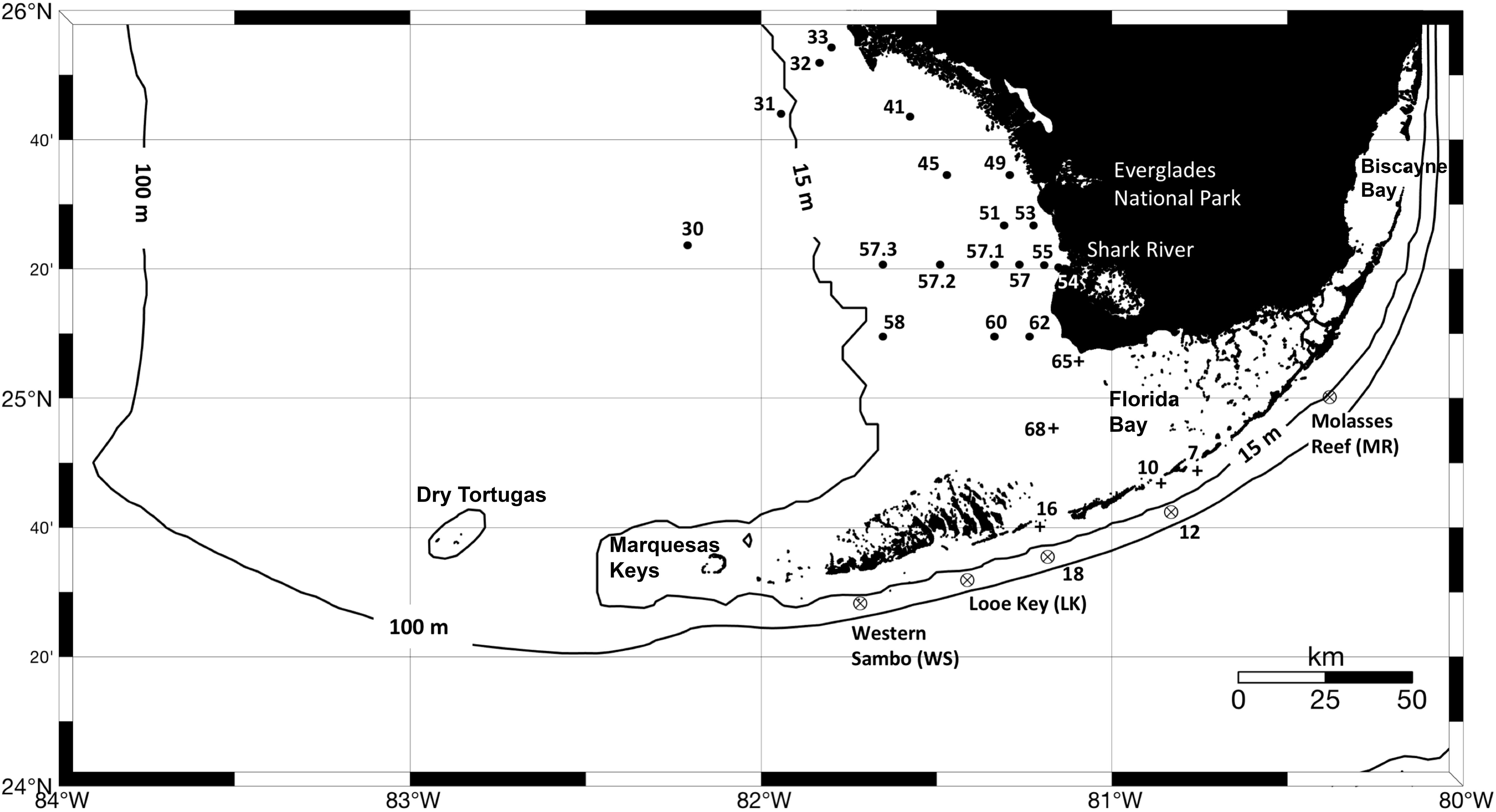
Figure 1. Location of sites sampled during the three oceanographic expeditions conducted in March, May, and September of 2016 led by the NOAA South Florida Program and the Marine Biodiversity Observation Network (MBON). Crossed circles indicate stations mostly occupied by oligotrophic waters, cross symbols indicate stations influenced by Florida Bay waters, and black circles show locations of sampled sites on the west Florida shelf. Measurements collected at each site include temperature, salinity, inorganic nutrients (DIN, SRP and Si), CDOM absorption at 443 nm [ag(443)], phytoplankton HPLC pigments, and filter pads for specific absorption of phytoplankton and non-algal particles (aphy and ad, respectively).
To compute the seascapes, we followed the classification approach of Kavanaugh et al. (2014). Briefly, climatological monthly means of SST, chl-a, and nFLH (2003–2010) were used as inputs to derive probabilistic self-organizing maps (PrSOM) (Anouar et al., 1998). The three variable spatio-temporal vectors led to 15 × 15 neuronal maps (i.e., 225 classes), each with its own 3-dimensional weight based on maximum likelihood estimation (3-D MLEs). The 3-D MLEs were reduced using a hierarchical agglomerative clustering (HAC) with Ward linkages (Ward, 1963). This method uses combinatorial, Euclidian distances that conserve the original data space with sequential linkages (McCune et al., 2002). The seascapes were then successively grouped until 90% of the variance was explained. This led to a total of 18 unique classes.
The 18 seascapes were numerically ordered according to the trophic state of each class. They increase from deep, offshore, oligotrophic conditions (class 1) to optically shallow, near-shore, eutrophic conditions (class 18; see Table 1). For example, seascape classes 1 through 3 correspond to water masses with very high SST (> 27°C) and very low chl-a values (<0.1 mg m–3). Classes 16 through 18 are indicative of water masses with the highest chl-a (> 1.8 mg m–3) and nFLH (>0.15 mW cm–2 μm–1 sr–1) values.
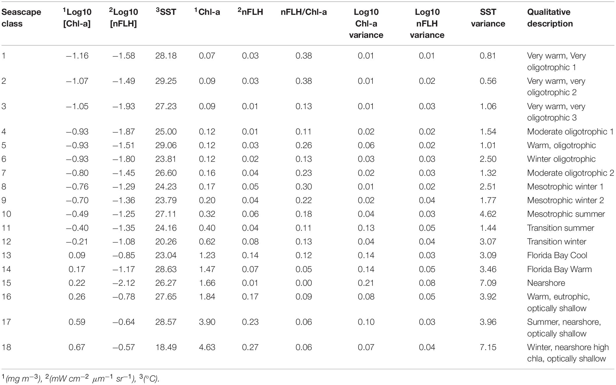
Table 1. Mean and variance values of satellite input data for each seascape class with corresponding qualitative description.
Once the spatial-temporal vectors were classified, the means, covariances, and proportion of total pixels classified within each seascape informed a multivariate Gaussian mixture model. Class assignments based on satellite data collected over each cruise duration were then determined by their maximum posterior probabilities.
To examine relationships between seascape classes and in situ observations, the dominant seascape class at each site sampled by ship was identified. Seascape values within a 3-pixel radius around each station were extracted using the Distance function of the Matlab software (Mathworks®), yielding ∼ 32 class values at each site depending on cloud cover or other possible masking. Therefore, a seascape class array could be composed by a particular combination of the 18 possible categories. In order to identify a predominant seascape category occupying each sampled site, a unique seascape value per station was obtained by calculating the distance-weighted geometric mean value () of the corresponding 32 class array, using the equation:
were x is the seascape value of the extracted pixel, and D is the inverse of the distance (geodetic arc length) between the center of the extracted pixel and the station location. Inverse distance values D were used to proportionally assign more weight to pixels closer to the stations. Weighted geometric means were employed to normalize differences in minimum and maximum seascape values amongst stations; some sites showed only one or two classes whereas other stations were surrounded by a higher number of seascape categories and thus showed more mixed conditions. The values were then rounded to the nearest unit for a final seascape classification assigned to each particular ship station.
In situ Measurements
Measurements of phytoplankton pigment concentration, hydrography, nutrient concentration, and inherent optical properties (light absorption coefficient by particulate and dissolved substances) were made from the R/V Walton Smith (University of Miami). Three expeditions were conducted in 2016: March 14–18 (WS16074), May 5–12 (WS16130), and September 19–23 (WS16263). A total of 24 stations were sampled for pigment concentration using High Performance Liquid Chromatography (HPLC) and bio-optical properties in March, 23 stations in May, and 27 stations in September. All cruises sampled waters around the Florida Keys, Florida Bay, and the west Florida shelf (Figure 1). The expeditions were conducted as part of the NOAA South Florida Ecosystem Restoration project [SFER; Atlantic Oceanographic and Atmospheric Laboratory (AOML)] and the Sanctuaries Marine Biodiversity Observation Network (MBON) field program.
Hydrographic data were collected using a Conductivity-Temperature-Depth (CTD) Sea Bird 911plus CTD system mounted on a rosette with twelve Teflon-coated 10-L Niskin bottles. The CTD was also equipped with Seapoint chlorophyll-a and colored dissolved organic matter (CDOM) fluorometers, a Biospherical Instruments 4-Pi Photosynthetically Available Radiation (PAR) sensor, and a WetLabs 25 cm transmissometer. Only the surface (1 m) data were used in this study to compare with satellite observations.
Surface concentrations of dissolved inorganic nitrogen (DIN, i.e., nitrate, nitrite and ammonia), soluble reactive phosphorus (SRP), and silicate (Si) were measured from samples collected directly from Niskin bottles. Nutrient samples were filtered through a 0.45 μm filter into 8-ml polystyrene test tubes that had been rinsed three times with the seawater to be sampled. The samples were stored frozen at −20°C until analysis at the Ocean Chemistry and Ecosystems Division of the AOML. Nutrients were measured on a SEAL Analytical autoanalyzer using standard gas-segment continuous flow colorimetric methods (Zhang and Berberian, 1997; Zhang et al., 1997, 2000; Zhang, 2000).
HPLC Pigment and CHEMTAX Analyses
Separate samples for HPLC, chlorophyll-a, and accessory pigment concentration measurements were collected by vacuum-filtering ∼ 0.1 – 2 L of seawater (depending on biomass concentration present) through a 25 mm glass fiber filter (Whatman GF/F, 0.7 μm pore size) on board ship. Filters were wrapped in aluminum foil and stored in liquid nitrogen. Once on land, HPLC samples were kept at −80°C until analyzed. HPLC analyses were conducted at the NASA Goddard Space Flight Center (GSFC), Maryland, following Van Heukelem and Thomas (2001) and Hooker et al. (2005). A total of 13 diagnostic HPLC pigments were recorded (Supplementary Table S1). All pigment data are available online at the NASA SeaWiFS Bio-optical Archive and Storage System (SeaBASS)2.
Of the pigment suite collected, seven diagnostic pigments (DP) were used to calculate the proportion of micro-, nano-, and pico-phytoplankton in a sample per Uitz et al. (2006):
Several diagnostic pigments in Supplementary Table S1 are unique to specific types of phytoplankton. For example, alloxanthin marks the presence of cryptophytes, and peridinin marks dinoflagellates. Most of the other pigments are present in more than one phytoplankton group (e.g., zeaxanthin is shared by cyanobacteria and chlorophytes). Since many algal groups have characteristic proportions of maker pigments, the relative abundance of specific taxa in a mixed phytoplankton population can be estimated using the ratio of individual diagnostic pigments (IP) to the sum of all diagnostic pigments (∑DP) or to total Chl-a (Mackey et al., 1996; Vidussi et al., 2001; Pinckney et al., 2015).
The relative abundances of chlorophytes, cryptophytes, cyanobacteria, diatoms, dinoflagellates, haptophytes, and prasinophytes were computed from pigment distributions using CHEMTAX v.1.95 chemical taxonomy software (Mackey et al., 1996; Wright et al., 1996). Specifically, relative abundances of two nominal sub-groups of cyanobacteria (Type 2 and 4), diatoms (Type 1 and 2) and haptophytes (Type 6 and 8), and of all remaining groups were derived following Pinckney et al. (2001, 2015) and Higgins et al. (2011) (Supplementary Table S2). Therefore, a total of ten phytoplankton groups were analyzed. CHEMTAX seeks to achieve an optimal fit to a matrix of phytoplankton taxa based on an initial IP:TChl-a ratio matrix (Supplementary Table S2). An initial limit matrix determines the extent to which each pigment ratio can be adjusted. We used the initial pigment ratio described in Higgins et al. (2011) with the default limit matrix included in CHEMTAX (Mackey et al., 1996) (see Supplementary Tables S2, S3). In this study we used the new CHEMTAX software (version 1.95), which runs multiple trials from randomized starting points that in turn generate 60 pigment ratio tables as described in Wright et al. (2009). To minimize errors resulting from inaccurate pigment ratio seed values, we separated the pigment data from each cruise into four bins using hierarchical cluster analysis (HAC; see section “Data Clustering and Statistical Analysis” and Supplementary Figure S1), and each sample group was run separately in CHEMTAX.
Inherent Optical Properties
Particulate Matter Light Absorption Coefficients
Samples were collected at each station for determinations of spectral absorption coefficients of total particulate matter and detritus [ap(λ) and ad(λ), respectively; in m–1]. We used the filter pad method of Mitchell and Kiefer (1988). Surface samples (0.1 to 2 L of seawater) from each station were vacuum-filtered through a 25 mm glass fiber filter (Whatman GF/F, 0.7 μm pore size) on board ship. After collection, filter pads were placed in Histoprep capsules and flash-frozen in liquid nitrogen until arrival to the laboratory, where they were transferred to a −80°C freezer. Filter pads were processed within 6 months of collection.
Spectral optical density [OD(λ)] was measured on the filters from 330 to 880 nm at ∼2 nm resolution using a custom-built, 512-channel spectrometer at the Optical Oceanography Laboratory of the College of Marine Science at University of South Florida. Initial OD measurements were used to estimate ap(λ) following the methods of Bricaud and Stramski (1990) and Mitchell and Kiefer (1988). After collection of ap(λ) spectra, filters were rinsed with hot (∼ 60°C) methanol for ∼ 20 min under low light conditions to extract phytoplankton pigments (Kishino et al., 1985; Roesler et al., 1989). Filters were then re-scanned for ad(λ) (non-algal particles; NAP) determinations. For each sample the difference between ap(λ) and ad(λ) was calculated to obtain the absorption coefficient of phytoplankton, aphy(λ).
Derivative analysis of phytoplankton absorption spectra was used to examine the relative dominance of diagnostic pigments in these mixed algal populations (Bidigare, 1989). This technique identifies absorption peaks of individual pigments using the second or fourth derivative of aphy. We computed vectors of the second derivative of aphy spectra (aphy”) using differences among consecutive waveband elements over the entire spectral range of the data. Spectral noise was removed from each aphy vector before computations of second derivative spectra by applying a least-squares smoothing filter (i.e., Savitzky-Golay) following Lorenzoni et al. (2015). Prior to calculating second derivative spectra aphy, vectors were normalized by the corresponding aphy value at 440 nm [i.e., aphy(λ)/aphy(440)]. This helps to remove some effects of Chl-a variability among samples (Nair et al., 2008).
We used the “finite approximation” technique to detect subtle changes in the spectral curvature between waveband elements or band separation (BS) (Torrecilla et al., 2009). BS between 5 and 10 nm yielded identical results. Thus, cluster analyses were constructed using a BS value of 9 nm as in Torrecilla et al. (2011). Matrices containing arrays of normalized aphy” spectra were then used in the cluster analysis to classify sampled stations.
Observations of phytoplankton light absorption at 492, 512, 550, and 673 nm and the concentration of photo-synthetic and photo-protective carotenoids provide information about phytoplankton community structure (Chase et al., 2013; Pinckney et al., 2015). We conducted least-square correlation analyses between these parameters using relative pigment concentrations values. Specifically, photosynthetic and photoprotective carotenoids [(PSC = but-fuco + fuco + hex-fuco + perid; PPC = allo + diadinoxanthin + diato + zea + alpha-carotenoid + beta-carotenoid)], as well as individual diagnostic pigments (e.g., zeaxanthin and fucoxanthin), were compared against aphy” minima centered at 492, 550 nm and 673 nm, and maxima centered at 512 with a linear regression model using the “fitlm” function in Matlab®. Negative correlation between aphy” values and pigment concentrations denote higher phytoplankton absorption with increasing pigment content, whereas positive correlations indicate lower phytoplankton absorption as a result of lower concentration of these pigments.
Dissolved Organic Matter Light Absorption Coefficients
Samples for colored dissolved organic matter (CDOM) absorption coefficient measurements were collected at each site by filtering 200 mL of seawater through a 47 mm Millipore membrane filter (0.2 μm pore size) using vacuum filtration. Samples were kept at ∼ 4°C until analysis within 2 weeks after collection. CDOM absorbance spectra, A(λ), were determined between 200 and 800 nm at ∼1 nm resolution using a Perkin Elmer Lambda 25 spectrophotometer equipped with 10-cm pathlength cells. Recently distilled Milli-Q water was used as a blank. The CDOM absorption coefficient (ag in m–1) was calculated with the following equation:
where r is the pathlength (10 cm). CDOM absorption values at 443 nm were used for analysis.
Data Clustering and Statistical Analysis
Hierarchical agglomerative cluster (HAC) analysis was employed for the classification of sampled stations based on HPLC diagnostic pigment and aphy” measurements (Figure 2). The HAC analysis uses an unsupervised algorithm that generates cluster trees (dendrograms) that group objects hierarchically according to pairwise distances between these objects. We utilized the Linkage function of the Matlab software (Mathworks®) to group stations occupied during each cruise. Specifically, we employed “Euclidian” distance as a metric to group objects (stations). The “average” method computes unweighted average distance between clusters. Dendrogram clusters were used to assess how station groupings during a field campaign related to seascape classes identified at each site (Figure 2). Input data to the HAC analysis consisted of matrices containing one numerical array per station. For example, the pigment matrix for the HAC analysis using data collected in the March cruise had 24 rows (stations) and 12 columns (pigment ratios).
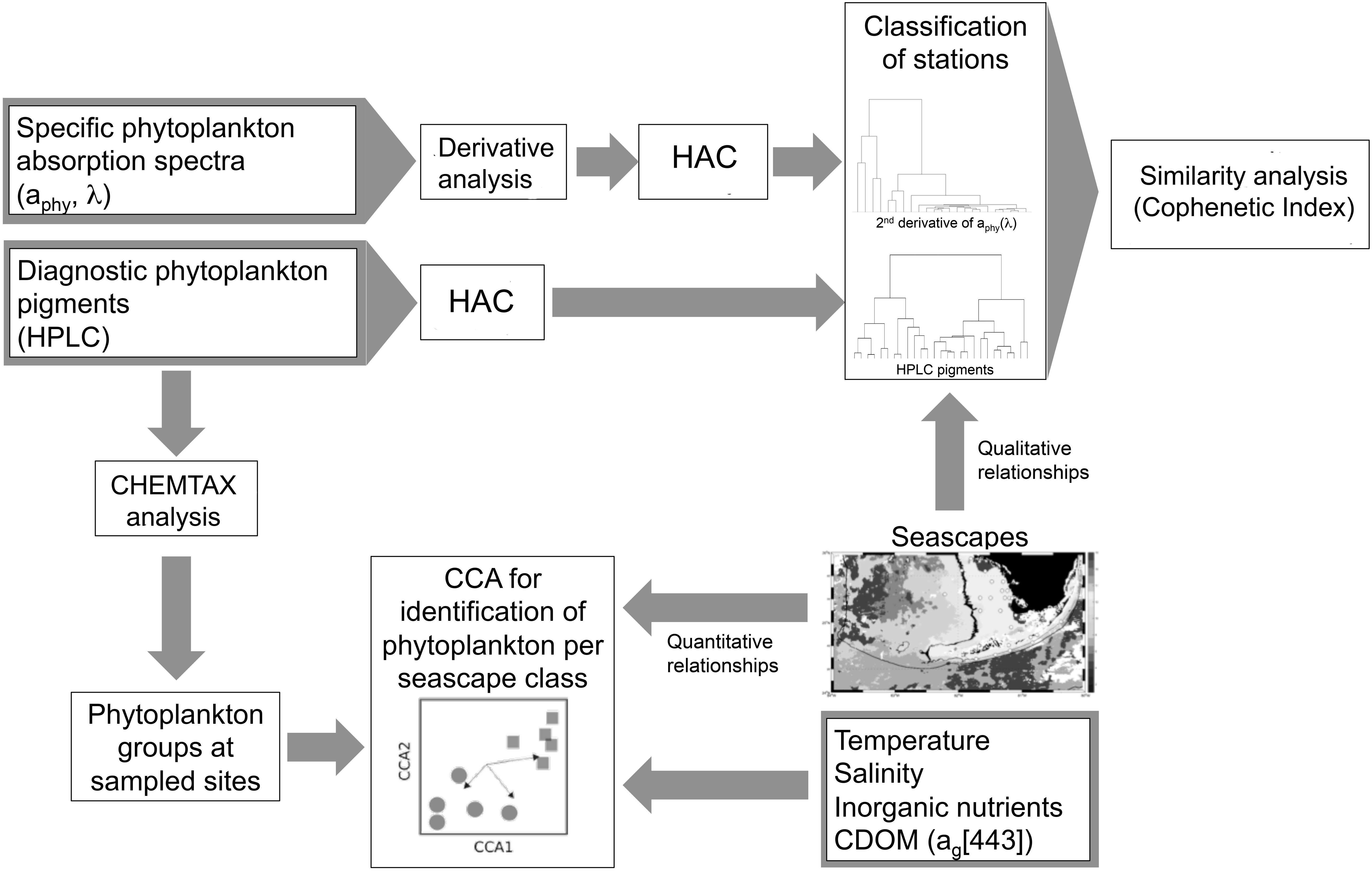
Figure 2. Schematic illustration of the study workflow for the identification of phytoplankton groups and aphy spectral signatures in sampled seascape classes based on hierarchical agglomerative clustering (HAC) analysis. Canonical correspondence analysis (CCA) was used to examine quantitative relationships between seascape classes, in situ environmental variables (temperature, salinity, nutrients, and CDOM), and phytoplankton groups derived from CHEMTAX analysis. Match-ups of station clusters derived from HAC analysis with corresponding seascape classes identified at sampled sites were conducted to unveil qualitative relationships between seascapes and phytoplankton proxy data (aphy spectra and HPLC pigments). To evaluate the extent to which phytoplankton community composition can be assessed with bio-optical data, similarity analyses were conducted using the cophenetic index to compare dendrograms generated with HPLC pigments versus those from aphy spectra.
Canonical correspondence analysis (CCA) were employed to identify relationships between pigment-derived phytoplankton taxa, environmental conditions (i.e., temperature, salinity, ag(443), and nutrients), and seascape classes. To facilitate interpretation of results we reduced the ten algal groups to seven classes by merging Diatoms Type 1 and 2, Cyanobacteria Type 2 and 4, and Haptophytes Type 6 and 8 into single corresponding groups. The CCA was performed using the statistical R software.
To examine relationships between the spatial distribution of phytoplankton based on pigment analyses and patterns in bio-optical data, we compared dendrograms constructed with aphy” vectors and those generated from HPLC pigment data using the cophenetic index as in Torrecilla et al. (2011) (Figure 2). This index represents correlation coefficient between cophenetic matrices of analyzed dendrograms and is proportional to the level of similarity of pairwise distances between data objects in each dendrogram. A cophenetic correlation coefficient of 1 means that dendrograms are identical.
Results
Seascape Classes
Seascape class values were derived for all stations that had complete datasets for all parameters of interest during the three cruises (Figure 3; see Figure 1 for station location). The lone exception was the pixel at Station 12 in March, 2016, which was obscured; therefore, the seascape value was assumed to be that of neighboring stations with similar oceanographic properties [i.e., Looe Key (LK) and Station 18].
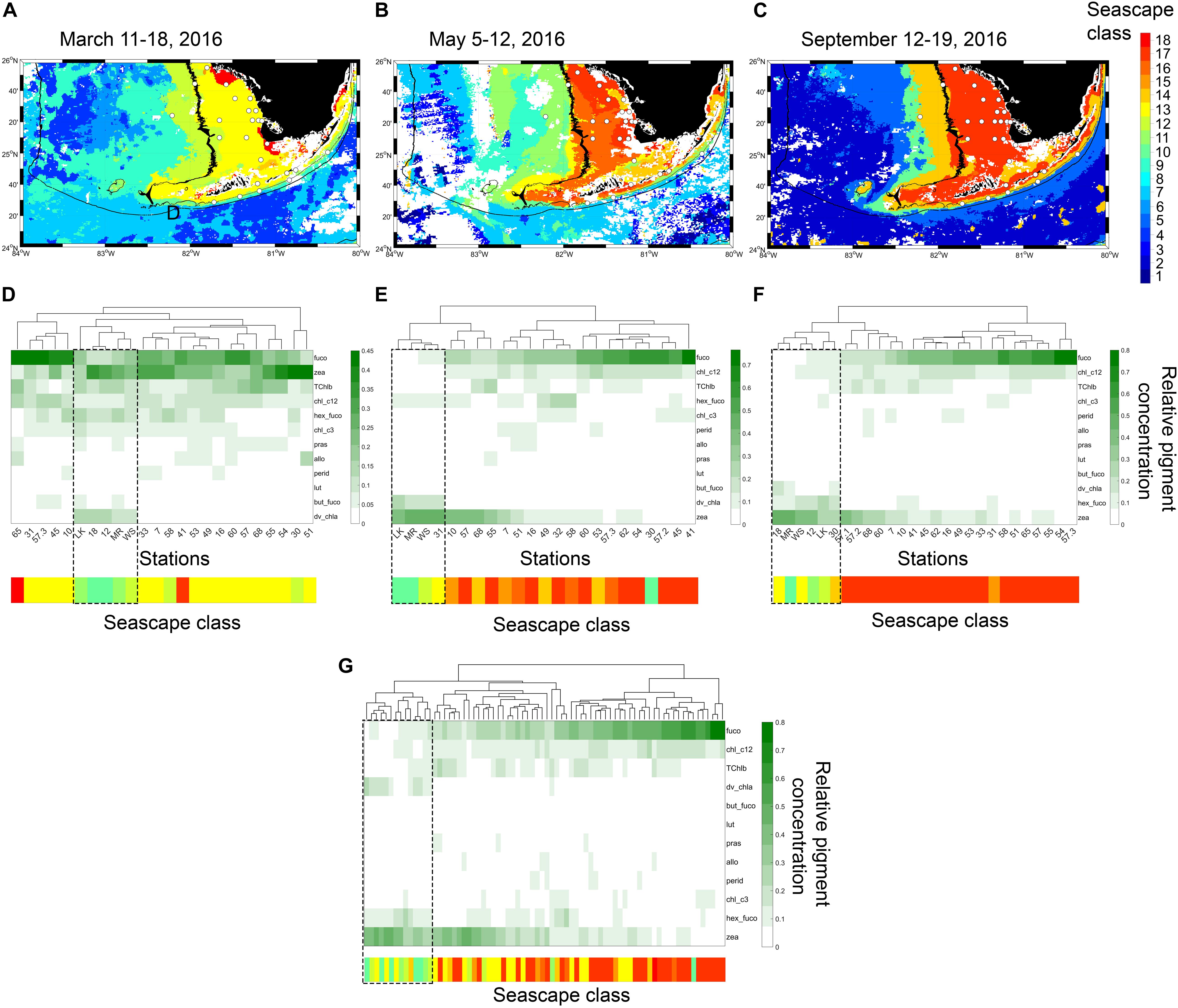
Figure 3. (A–C) Eight-day composite seascape maps during each cruise with sampled stations shown with white dots. The 15 and 100 m isobaths are shown with black lines at 30 s spatial resolution. (D–F) dendrogram clustering of sampled stations derived from HAC analysis of pigment data (HPLC) for each sampling period. Heat maps below dendrograms show fractional proportions of specific diagnostic pigments relative to the sum of all diagnostic pigments at each site (note that color scale changes between sampling periods). Row labels in heat map are pigment abbreviations described in Supplementary Table S1. Column labels in heat map correspond to station ID’s shown in Figure 1. Color bars below heat maps indicate seascape class identified in each station during corresponding cruises. Dashed rectangles highlight clustering of stations where Mesotrophic and Transition seascapes (classes 10 through 12; Table 1) are dominant classes. (G) dendrogram clustering constructed with combined data from the three cruises.
During the March 2016 cruise, six dominant seascape classes were identified across the 24 sampled stations (Table 2). The Florida Bay Cool seascape (class 13) was the dominant class in ∼ 63% of stations, most of which were located within the 15 m isobath across the west Florida Shelf (Figure 3). Moderate Oligotrophic 1 through Transition Winter seascapes (i.e., seascapes with values < 13; see Table 1 for seascape description) were detected in ∼ 30% of stations, mostly in deeper waters of the west Florida Shelf and along the reef track. During the May and September cruises, mean seascape conditions at sampled stations corresponded to eight classes between class 10 and 17. In May, ∼ 65% of stations occupied were optically shallow seascape classes 16 and 17 mostly over the Florida Bay and west Florida shelf waters with depths <15 m. All other sites in May exhibited more mixed seascape conditions. In September, 74% of stations had optically shallow seascape class 17 over the west Florida shelf, while Mesotrophic, Transition and Florida Bay seascapes (classes 10 through 14) were observed at all other stations.
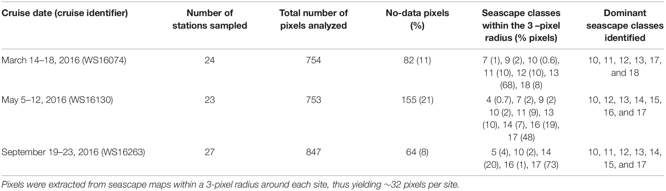
Table 2. Seascape classes identified across all sampled stations during the three field campaigns.
The dominant seascape classes detected at stations near the 100 m isobath along the southern side of the Florida Keys (gray squares in Figure 1) during the three sampling periods varied between Mesotrophic Summer and Florida Bay Cool (classes 10 and 13, respectively; see Table 2). Florida Bay stations (crosses in Figure 1) typically had seascapes classes ranging from Florida Bay Cool (class 13) to Winter, Nearshore High Chla, Optically Shallow (class 18) over the same period. The west Florida shelf stations (black circles in Figure 1) exhibited higher seascape variability (Transition Summer [class 11] through to Summer, Nearshore, Optically Shallow [class 17]; see Table 2).
Types of Phytoplankton Pigments in Different Seascapes
On average, Fucoxanthin (Fuco), Zeaxanthin (Zea), Chlorophyll c1 + c2 (Chl_c12), total chlorophyll b (TChlb) and 19′-hexanoyloxyfucoxanthin (Hex-fuco) represented 82% of the total pigment pool in all samples collected during the three cruises. Fucoxanthin and zeaxanthin accounted for 54% of the total pigment assemblage. Hex-fuco was generally the fifth most abundant pigment in all sampling periods. Relative contributions of chlorophyll c3, prasinoxanthin, alloxanthin, 19′-butanoyloxyfucoxanthin and lutein to the total pigment pool did not show a clear relationship with seascape class.
Stations grouped based on similar HPLC pigment composition (HAC analysis) allowed inferences to be drawn about phytoplankton community composition in different seascapes (Figure 3). During the three field campaigns, stations occupied by Mesotrophic Summer through Transition Winter seascapes (classes 10 – 12) typically grouped within the same pigment clusters, an indication that they had similar phytoplankton communities (see section “Phytoplankton Assemblages in Sampled Seascapes” for description of phytoplankton communities). The exceptions were stations 58 and 30 in March, and station 30 in May. These did not cluster with those also occupied by the same seascape classes (10 through 12) possibly because these sites were located at or near the boundary of higher category seascapes.
High-performance liquid chromatography groupings in Florida Bay and Nearshore seascapes (classes 13 – 15) displayed a weaker correlation; these pigment clusters often spanned different seascapes (e.g., see May cruise; Figure 3). Pigment composition of stations in optically shallow seascapes (classes 16 – 18), here defined as seascapes with the highest chl-a and nFLH values (see Table 1) that were typically present over shallow areas, generally showed consistent differences with respect to stations in Mesotrophic and Transition seascapes (classes 10 – 12). The HAC algorithm identified typical pigment groups in Eutrophic, Optically Shallow seascapes.
In general, the lowest relative fucoxanthin and chlorophyll c1 + c2 concentrations were observed in Mesotrophic Summer through Transition Winter seascape (classes 10 – 12; Figure 3). Fucoxanthin in Nearshore to Optically Shallow seascapes (classes ≥ 15) was nearly three-fold higher than in Mesotrophic and Transition seascapes, and two-fold higher than in Florida Bay seascapes (classes 13 and 14; Figure 3). Chlorophyll c1 + c2 showed a similar pattern. TChlb was ∼ 28% higher in seascapes ≥13 than lower seascape classes. Hex-fuco fractions were between 8 and 48% lower in samples collected in seascapes ≥13 than lower seascapes classes. Zeaxanthin values were nearly two-fold higher in seascapes ≤13 than seascape classes 14 to 18 (Florida Bay Cool to Optically Shallow).
Divinyl chlorophyll a (DVChl-a), a diagnostic pigment of the cyanobacteria Prochlorococcus spp. (Cyanobacteria Type 4), was undetected in stations occupied by Nearshore through Optically Shallow seascapes throughout the study period (Figure 3). DVChl-a values observed in seascapes <13 during March and May cruises were three to 79-fold higher than in seascapes 13 and 14. During the September cruise, however, DVChl-a was ∼40% higher in seascapes 13 and 14 than seascapes classes 12 and lower.
Peridinin, a pigment diagnostic of dinoflagellates, was generally observed at low concentrations across all seascape classes. Relative pigment concentration values of peridinin ≥0.1 were only measured in Nearshore and Optically Shallow seascapes in May (stations 7 and 16), and only in Optically Shallow seascapes in September (stations 7 and 49; Figure 3). Peridinin in seascape classes ≥ 14 were, on average, ∼ 40% higher than in lower seascape classes.
Phytoplankton Assemblages in Sampled Seascapes
There were consistent relationships between seascapes, phytoplankton size classes, and taxa observed in the three expeditions (Supplementary Figure S2). The relative contributions to total Chla [(TChla)] of micro-phytoplankton (>20 μm size class) increased from ∼ 24% in Mesotrophic Summer seascapes (class 10) to ∼ 70% in Winter, Nearshore High Chla, Optically Shallow seascape (class 18; Figure 4).
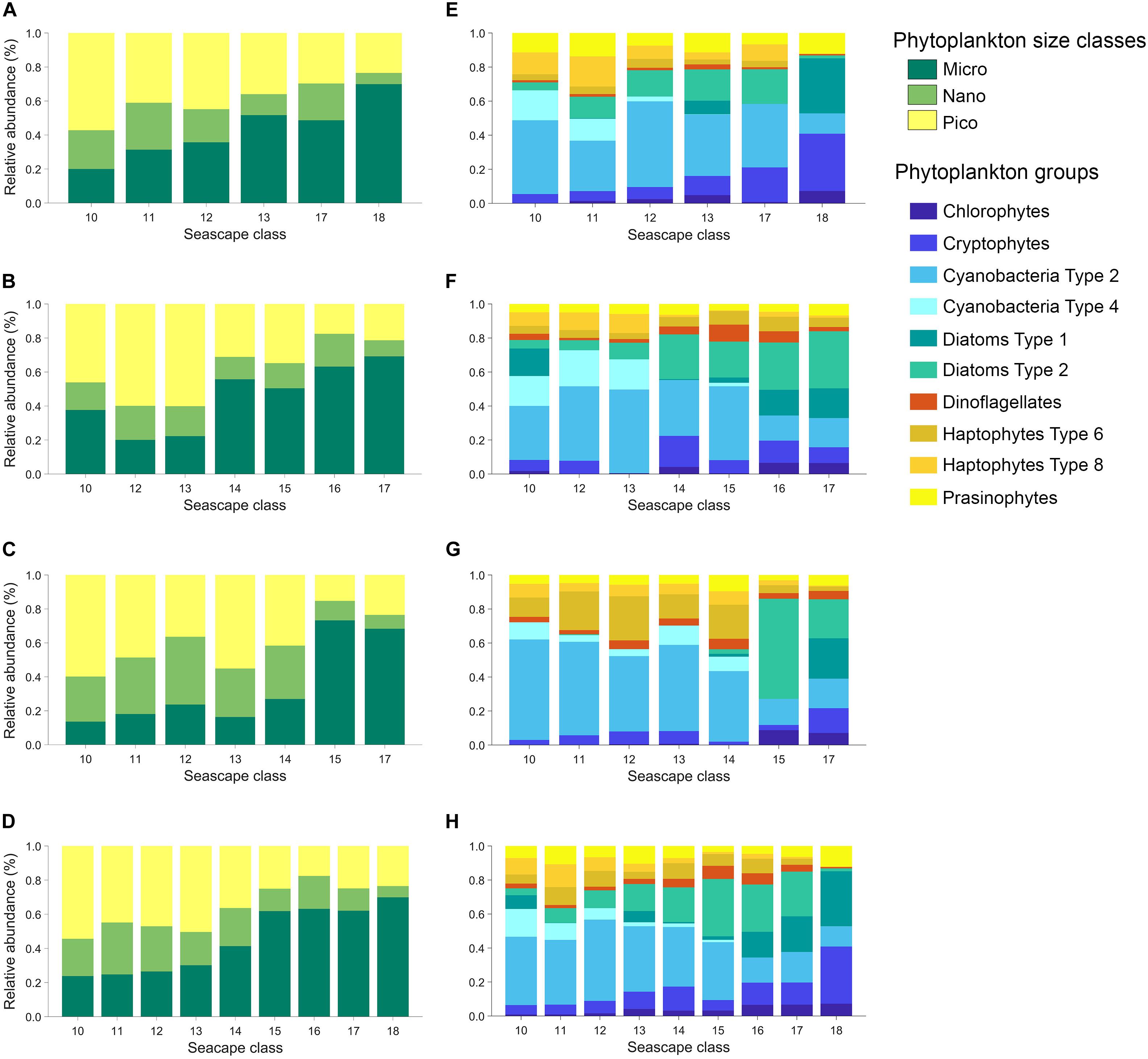
Figure 4. Left: Average contribution of phytoplankton functional types (PFT: micro-, nano-, and pico-phytoplankton) to total chl-a (TChla) derived from diagnostic HPLC pigments using equations described in Uitz et al. (2006) estimated for each seascape class during March, May, and November 2016 cruises (A–C), and for all the data combined (D). Right: Average community composition of ten phytoplankton groups estimated for each seascape class derived from CHEMTAX analysis during March, May and November 2016 cruises (E–G), and for all the data combined (H).
The opposite was observed with pico-phytoplankton (<2 μm). They showed ∼ 55% relative chl-a biomass in Mesotrophic Summer seascape (low chl-a; see Table 1) and steadily decreasing to ∼ 24% in Optically Shallow seascapes (high chl-a). Minimum and maximum pico-phytoplankton relative biomass were observed in Optically Shallow seascapes (∼18% in class 16) and Mesotrophic Summer (∼ 55% in class 10), respectively. Similar results, but with greater uncertainty, were obtained with relative biomass of nano-phytoplankton (2 – 20 μm). Nano-phytoplankton was lowest in Optically Shallow seascapes (∼ 7% in class 18) and highest in mesotrophic and Transition seascapes (∼ 30% in class 11).
Cyanobacteria dominated in Mesotrophic Summer through Florida Bay Cool seascapes (classes 10 – 13) with mean relative contributions to TChla ranging from ∼ 57% to over 60% (Figure 4 and Supplementary Figure S2). Cyanobacteria also dominated in Florida Bay Warm seascape (class 14) but their contribution to TChla dropped to ∼ 38% in this class. Specifically, Cyanobacteria Type 4 as indicative of Prochlorococcus spp. was only present in Mesotrophic Summer through Florida Bay Cool seascapes. The exception was observed at Station 30 where Prochlorococcus was detected during the September cruise when the site was occupied by Florida Bay Warm (class 14). The relative biomass contribution of this phytoplankton group decreased steadily in higher seascape classes to a minimum of about ∼ 11% (Optically Shallow class 18). Haptophyte relative biomass also appeared to be higher in the lower seascape classes (10 – 12) than in higher ones, and their contributions to TChla never exceeded ∼ 24%.
Diatoms showed lower contributions to TChla in Mesotrophic and Florida Bay seascapes (<10% in classes 10 to 13) and significantly increased in Florida Bay Warm and Optically Shallow (∼ 36% in classes 14 to 18; Figure 4). Cryptophytes and chlorophytes showed a similar distribution, with higher relative biomass with increasing seascape class. Cryptophytes contributed ∼ 5 to 29% to total chl-a pool (seascapes 10 and 18, respectively). Minimum and maximum relative biomass of chlorophytes were ∼ 3 and 10% observed in seascapes 11 and 18, respectively.
The relative biomass of dinoflagellates and prasinophytes did not show a clear relationship with seascape class. These organisms were present at low concentrations in every class (Figure 4 and Supplementary Figure S2). For example, the relative biomass of dinoflagellates ranged between ∼ 2% in Mesotrophic and Transition Summer seascapes (classes 10 and 11) and ∼ 6% in Florida Bay Warm seascapes (class 14), and those of prasinophytes oscillated between ∼ 3% in Nearshore seascapes (class 15) and ∼ 11% in all higher seascape categories.
Seascapes and Inherent Optical Properties
Analysis of the derivative of the absorption coefficient of phytoplankton (aphy) spectra (see section “Inherent Optical Properties”) allowed us to identify dominant phytoplankton in different seascapes. Differences in the shape of the second derivative of aphy (here denoted as aphy”) between 450 and 550 nm, and also at 673 nm (Figure 5), were especially apparent between seascapes. The lowest minima in aphy” were observed at ∼492 nm and the highest maxima at ∼512 nm in Mesotrophic and Transition seascapes (classes 10 – 12). A statistically significant inverse relationship between PPC and aphy(492)” (rppc–492 = 0.53; p < 0.001; n = 74) was also found. A weaker correlation was observed between zeaxanthin levels and aphy(492)” values (rzea–492 = 0.44; p < 0.001; n = 74). Zeaxanthin and PPC showed a significant positively correlation to a peak in aphy(512)” (rzea–512 = 0.62 and rppc–512 = 0.63; p < 0.001; n = 74).

Figure 5. Upper: Band-normalized phytoplankton absorption spectra [aphy(λ)/aphy(440)] from March, May and September cruises in 2016 (A–C), respectively) of three seascape class groups: Mesotrophic and Transition seascapes (classes 10–12) in green, Florida Bay, and Nearshore seascapes (classes 13–15) in yellow, and Optically Shallow seascapes (classes 16–18) in red. Middle: Second derivative of aphy(λ)/aphy(440) for corresponding cruises for all sampled sites and averaged by seascape class. Lower: Dendrogram clustering of sampled stations derived from HAC analysis of second derivative of aphy(λ)/aphy(440) for each sampling period. Dendrogram labels correspond to station ID’s shown in Figure 1. Bottom dendrogram (D) shows groupings of second derivative of aphy(λ)/aphy(440) spectra using data from all sampling periods combined. Dendrogram leaves are color coded according to seascape class identified in each station during corresponding cruises. Black arrows indicate aphy(λ)” troughs at 492, 550, and 673 nm, and the aphy(λ)” peak at 512.
PPC and zeaxanthin relative concentrations tended to be higher in Mesotrophic Summer through Transition Winter seascapes (class 10 – 12) than in higher seascape categories. Both minima at 492 nm and maxima at 512 nm became progressively smaller with increasing seascape value, from Florida Bay through Optically Shallow seascapes. The aphy” values in Nearshore seascapes (class 15) or higher were consistently less variable within the 450 and 550 nm region than those of lower classes during the three cruises (Figure 5). Differences in aphy” minima between seascape classes were also found in the 600 – 700 nm region, which is strongly affected by the chl-a red absorption peak. Large minima around 673 nm were typically observed in samples collected in Optically Shallow seascapes. Seascape classes of lower trophic state (e.g., Mesotrophic classes) showed less pronounced troughs; the lowest minima of aphy” at 673 nm were observed in Mesotrophic Summer through Transition Winter seascapes.
Our results indicate distinct phytoplankton spectral absorption signatures across seascape classes. HAC cluster analysis using aphy” spectra revealed groupings of seascape classes similar to those obtained with HPLC pigment data. Mesotrophic and Transition seascapes (classes 10 – 12) along the Florida Keys reef tract and some offshore stations (i.e., stations 58 and 30; Figure 1) generally matched pigment-based HAC clusters (Figure 5). Stations occupied by Florida Bay and Nearshore seascapes (classes 13 – 15) were also generally clustered together by the HAC algorithm. The largest linkage distances were observed between groups represented by Mesotrophic and Transition seascapes (<13) and those of Optically Shallow classes (>15).
Seascapes also showed clear differences in CDOM spectral absorption (ag) curves (Supplementary Figure S3). The ag at 443 nm (blue) generally increased progressively with increasing seascape number (i.e., moving toward the coast and in river-influenced areas). ag(443) values measured in Florida Bay, Nearshore and Optically Shallow seascapes (classes 13 through 18) typically observed on the coastal zone of Florida Bay and west Florida shelf and around areas affected by freshwater discharge from the Everglades were ∼ 2 to 20-fold higher than in Mesotrophic and Transition seascapes (classes 10 – 12) along the Florida Keys reef tract, Florida Straits, and in deeper offshore waters.
Figure 6 shows total absorption values of particulate and dissolved phases, namely phytoplankton absorption (aphy), non-algal particles (ad) and CDOM (ag), and the fractional contributions of these individual constituents to total absorption at 443, 555, and 673 nm wavelengths for sampled seascape classes. Light absorption at 443 nm observed in Mesotrophic and Transition seascapes (classes < 13) was mainly affected by phytoplankton and CDOM. The contribution of non-algal particles to the absorption budget in these classes was negligible (< 10%), except at 555 nm where ad reached maximum fraction of ∼ 25%. In Florida Bay and Nearshore seascapes (classes 13 – 15), CDOM showed the highest contribution to total absorption in the 443 and 555 nm bands, followed by aphy. The same was observed in Optically Shallow seascapes (classes > 15), where also the highest contributions from non-algal particles were measured with values of up to ∼ 40% (at 555 nm). Phytoplankton was the dominant constituent affecting ∼ 50 – 100% of the absorption budget at 673 nm in all seascape classes.
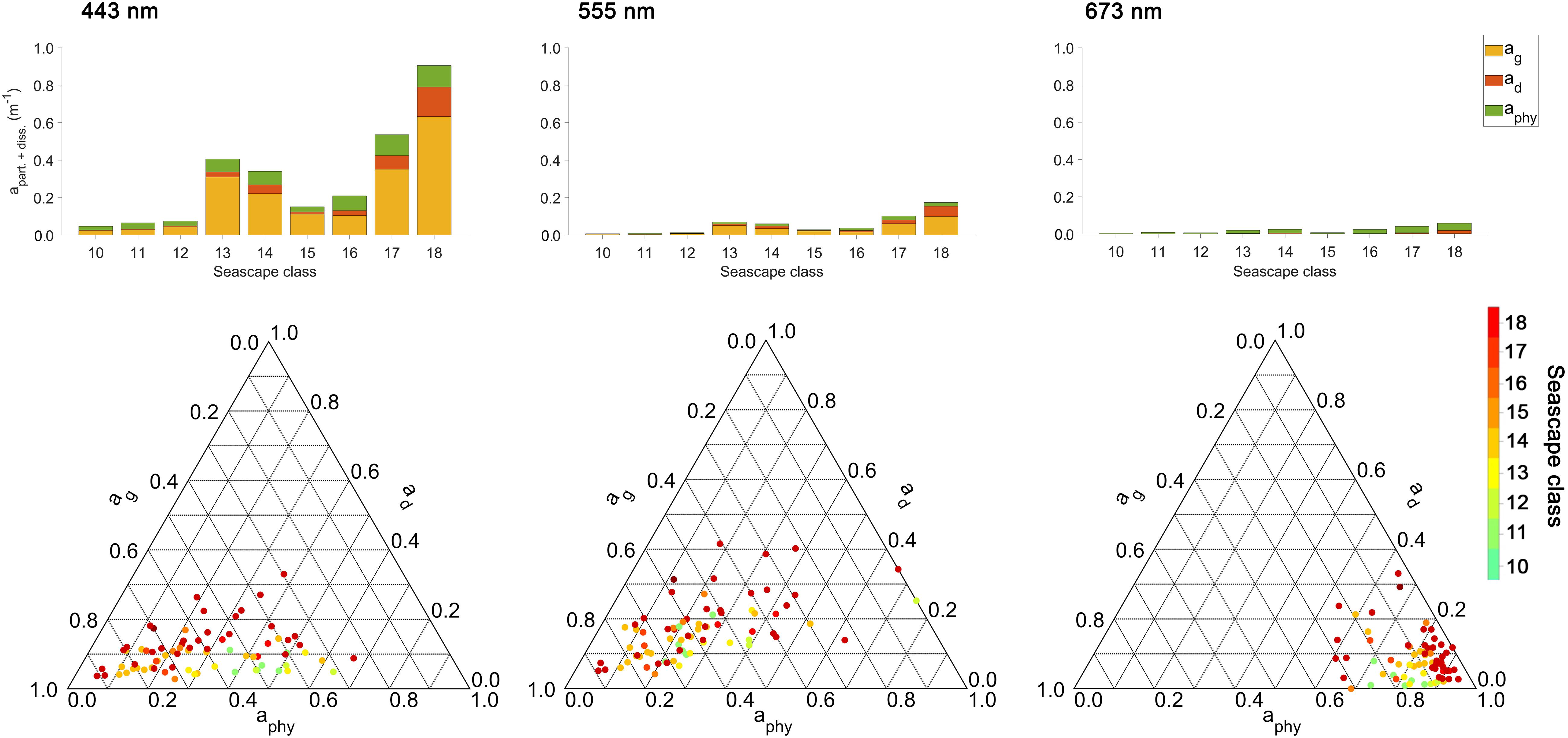
Figure 6. Absorption budgets for particulate and dissolved phases of individual seascape classes at 443, 555, and 675 nm bands. The top row shows absorption levels of particulate and dissolved components measured in sampled seascape classes at corresponding bands. The bottom row shows distributions of fractional absorption coefficients for phytoplankton (aphy), detritus (or non-algal particles; ad), and Colored Dissolved Organic Matter (CDOM; ag) and corresponding wavelengths above [ternary plots generated using (Ulrich, 2020)].
Canonical correspondence analysis indicate that the lower Mesotrophic through Transition seascape classes showed distinct phytoplankton communities compared to higher categories (Figure 7). Except for May, these classes formed statistically significant clusters generally associated with cyanobacteria and haptophytes, and larger taxa like diatoms and chlorophytes (ANOSIM rMarch = 0.4 and rSeptember = 0.48; both with p < < 0.01). In March these classes also showed a consistent affinity with higher salinity and lower CDOM values indicative of oceanic conditions; statistical relationships between Mesotrophic through Transition seascape, and SST, salinity and nutrients were significant at p < 0.01 (Figure 7). These seascapes (classes 10–13) were generally associated with high relative proportions of Prochlorococcus spp. (Cyanobacteria Type 4) almost exclusively, and haptophytes (Supplementary Figure S2).
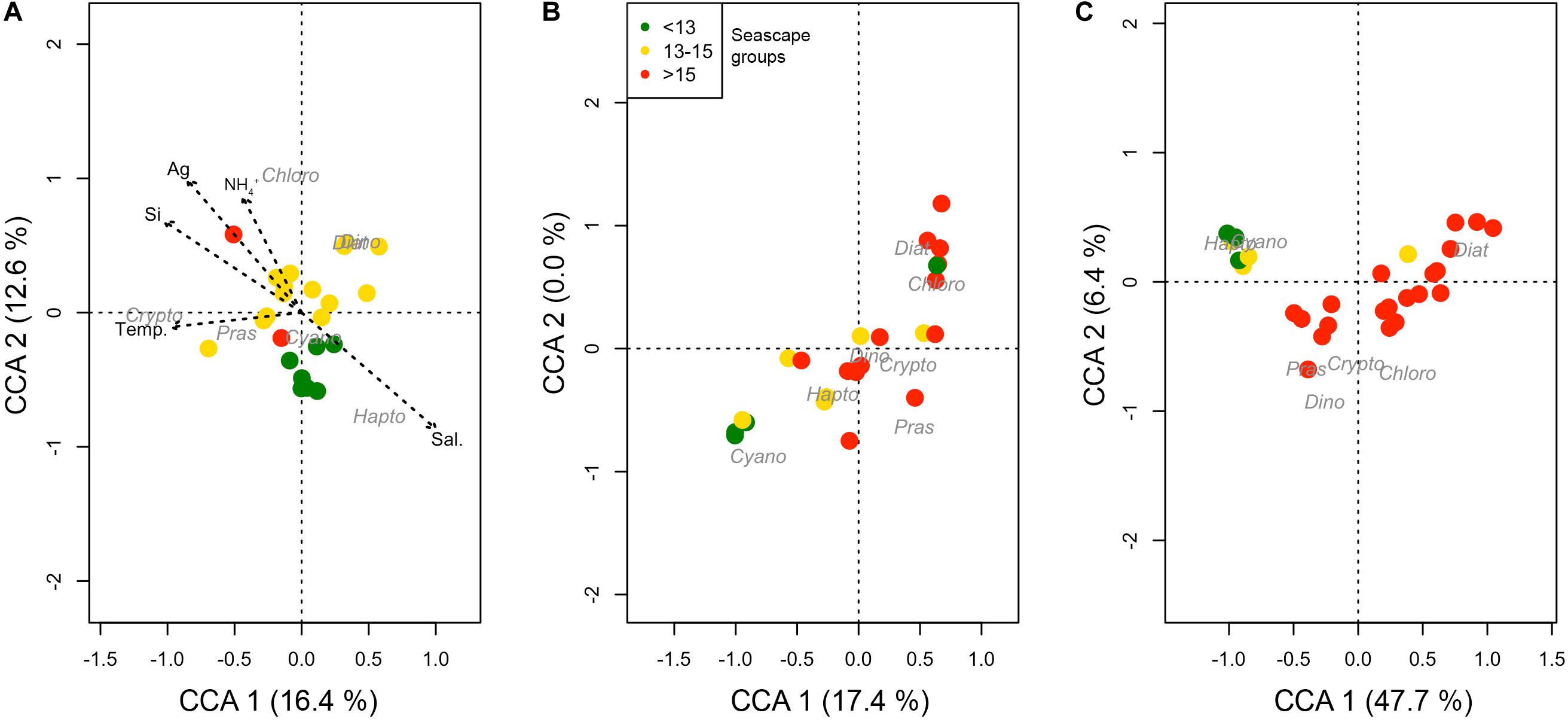
Figure 7. Coordinate correspondence analysis (CCA) of phytoplankton groups based on CHEMTAX outputs and hydrographic variables [temperature, salinity, inorganic nutrients and ag(443) for March, May, and September 2016 (A–C), respectively]. Dot color represents seascape group (classes < 13 in green, 13–15 in yellow and >15 in red) identified at the corresponding station for each observation. Arrows are plotted only for March 2016, when a statistically significant (p-value < 0.05) relationship between environmental variables, phytoplankton groups and seascape class was found.
Similarity among cluster trees obtained from aphy” coefficients versus pigment measurements varied depending on the spectral region examined. Cophenetic correlation analysis revealed high similarity levels (>0.5) in pairwise comparisons between dendrograms constructed with aphy” arrays and reference HPLC-derived dendrograms within narrow spectral bands (5 – 10 nm), notably in the violet through yellow and orange regions (440 – 540 and 640 nm, respectively; Supplementary Figure S4). The highest cophenetic correlation indices (∼ 0.9) were observed in May when comparing cluster trees derived from seascape class distributions and aphy” dendrogram trees as reference, in similar spectral regions covering blue through yellow bands (450–540 nm, respectively).
Discussion
Phytoplankton Pigments and Inherent Optical Properties of Seascapes
CHEMTAX and bio-optical results agree and show that: 1) nano- and pico-phytoplankton dominate in more oceanic and clear waters (lower seascape classes, < 13), that 2) larger taxa dominate in nearshore areas (higher seascape classes, > 15), and that 3) intermediate seascapes contain mixed communities (classes 13 – 15; Figure 4). Mixed phytoplankton assemblages were found in Florida Bay Cool and Warm, and Nearshore seascapes with balanced relative proportions of pico-, nano- and micro-phytoplankton taxa (Figure 4). Comparable proportions of pico- and micro-phytoplankton (41% and 36%, respectively) were measured in Florida Bay Warm seascape (class 14), with similar relative abundances of cyanobacteria, diatoms, and dinoflagellates.
As expected, the Optically Shallow seascape categories (classes > 15) appeared to cluster around communities dominated by larger taxa like diatoms, dinoflagellates and chlorophytes. Fast-growing large phytoplankton can be expected in these classes since these typically occupy very shallow areas likely exposed to higher runoff and nutrient inputs (Nunes et al., 2018). Furthermore, we found that Synechococcus spp. and Prochlorococcus spp. (Cyanobacteria Type 2 and 4, respectively) are well represented, or dominate, assemblages of oceanic Mesotrophic and Transition (classes 10–12) and Florida Bay Cool (class 13) seascapes. Prochlorococcus spp. in particular was observed in these seascapes almost exclusively (Figure 4 and Supplementary Figure S2); Mesotrophic and Transition classes are characterized by high salinity and low nutrient conditions under which cyanobacteria typically thrive (Mojica et al., 2015; Nunes et al., 2018). Vaillancourt et al. (2018) also found positive correlations between the cyanobacterium Prochlorococcus spp. and high salinity and nutrient-poor waters, whereas eukaryotic phytoplankton typically dominate in cooler and nutrient-rich areas. As in this study, they observed that cyanobacteria tend to cluster separately from eukaryotic phytoplankton in response to nutrient levels driven by temperature gradients and water column stratification. These findings are also consistent with results from previous studies describing HPLC-based phytoplankton assemblages across hydrographic or biogeochemical provinces in the Atlantic Basin (Gibb et al., 2000; Aiken et al., 2009; Torrecilla et al., 2011; Lorenzoni et al., 2015; Barlow et al., 2016; Araujo et al., 2017).
Results from spectral analyses confirmed phytoplankton assemblages derived from pigment observations. We identified a significant correlation between aphy(492)” minima and PPC relative concentrations, including zeaxanthin, possibly as a result of increasing dominance of small phytoplankton, i.e., Synechococcus spp. and Prochlorococcus spp., in lower seascape classes (Mesotrophic Summer through Transition Winter), which identify more offshore waters with lower nutrient and CDOM loads (Figure 5). Previous studies in this region have shown that high PPC concentrations associated with cyanobacterial blooms of Synechococcus spp. dominate the phytoplankton absorption budget at the 490 nm spectral band (Cannizzaro et al., 2019). A similar statistical relationship between aphy(492)” and DVChl-a was also observed in these classes, indicating dominance of the cyanobacteria Prochlorococcus spp specifically in these classes.
Higher aphy” (thus lower phytoplankton absorption) at 512 nm were observed with increasing relative concentrations of these pigments in Mesotrophic Summer through Transition Winter seascapes. In Optically Shallow seascapes (classes > 15), where zeaxanthin and PPC had lower relative concentrations, aphy” spectra tended to be flatter around the 512 nm band (Figure 5). This spectral band is in the vicinity of the aphy peak of PSC centered at 523 reported by Chase et al. (2013) and thus higher phytoplankton absorption at 512 nm can be expected when the abundance of diagnostic pigments of large taxa such as diatoms (fucoxanthin) or dinoflagellates (peridinin), increases. These results are further supported by significant negative correlations observed between PSC and aphy(512)” (r = 0.62; p < < 0.001).
Comparable high correlations between PPC and aphy(550)” peak values were also observed, providing further evidence of increased dominance of small phytoplankton in Mesotrophic Summer through Transition Winter seascapes (Figure 5). This is consistent with findings by Chase et al. (2013, 2017) using data from the Atlantic, Pacific and Indian ocean basins, and results by Lorenzoni et al. (2015) from the Cariaco Basin, Venezuela, collected by the CARIACO Ocean Time Series program (Muller-Karger et al., 2019), and Cannizzaro et al. (2019) from observations in Florida Bay.
Inverse correlations were observed between fucoxanthin and aphy(673)” (r = 0.46; p < 0.001), likely driven by dominance of large taxa with increasing seascape class (Figure 5); fucoxanthin is a diagnostic pigment of large phytoplankton groups such as diatoms. Several other studies have found a consistent effects of diatom concentrations on aphy spectra at this wavelength or in its close vicinity across different ocean regions (Werdell et al., 2014; Lorenzoni et al., 2015; Catlett and Siegel, 2018; Reynolds and Stramski, 2019).
Phytoplankton Spectral Characterization of Seascapes
Light absorption in sampled seascapes was mostly affected CDOM concentration and phytoplankton at spectral bands known to capture information about diagnostic pigments, i.e., 443, 555 and 673 nm wavelengths (Figure 6). In all three bands aphy accounted for a significant portion of the absorption budget across all seascapes, and most notably at the 673 nm band where phytoplankton (aphy) often dominated > 90% of the light absorption. Similar results were found in studies carried out in the western Arctic Ocean (Reynolds and Stramski, 2019), Mediterranean Sea (El Hourany et al., 2019b) and the tropical and subtropical eastern Atlantic Ocean (Taylor et al., 2011; Torrecilla et al., 2011).
To determine the degree to which phytoplankton absorption properties and phytoplankton communities can be represented by seascapes, we compared dendrograms generated from pigment data and aphy” spectra using the cophenetic correlation coefficient, a similarity metric (Taylor et al., 2011; Torrecilla et al., 2011). This pairwise comparison was carried out using HPLC-derived dendrograms as a reference versus those constructed with varying combinations of spectral ranges of aphy” curves (Methods). The rationale is that PSC and PPC affect aphy” peaks computed across narrow (∼ 5–10 nm) spectral bands, e.g., PPC in the 490 – 500 nm region and PSC in the 510 – 520 nm region (Chase et al., 2013). Thus, dendrogram trees constructed with data from more constrained spectral bands should have a higher similarity to corresponding reference HPLC trees than those using the entire spectral range (400 – 800 nm).
Although the degree of similarity between pigment and aphy” dendrogram clusters varied among cruises, the highest cophenetic index (∼ 0.5 – 0.6 in March and September cruises, and ∼ 0.3 in the May cruise) was generally found in the 440 (violet) and 640 nm (orange) spectral regions (Supplementary Figures S4A–C). The highest similarity between pigment-based and aphy” dendrogram trees was observed in the ∼ 480 – 570 nm spectral range, consistent with results from the eastern Atlantic Ocean (Taylor et al., 2011). These are somewhat modest cophenetic index values, but they are likely a result of statistical biases from relative oversampling of Florida Bay Warm and Summer, Nearshore, Optically Shallow seascapes classes (13 and 17, respectively) with respect to lower trophic state Mesotrophic and Transition seascapes (classes 10 – 12). Indeed, 66% of our samples came from seascapes classes 13 and 17 versus 19% in seascape classes 10 through 12.
Low cophenetic correlation between pigment and aphy” dendrogram trees could be attributed to high similarity among spectra collected in Florida Bay seascapes (13 and 14), and those of lower and higher seascape classes. For example, aphy” spectral curves from seascapes 13 – 15 were often indistinguishable from those collected in seascapes classes 16 – 18 during the March cruise and classes 10 – 12 during the September (Figure 5). This further supports the notion that Florida Bay seascapes carry a mixture of phytoplankton taxa also present in lower and higher seascapes. These actually have similar bio-optical characteristics with similar aphy” spectral curves, therefore affecting the performance of the clustering algorithm. Higher similarity among aphy” and pigment cluster trees could be expected if data collected over a wider range of seascape classes with a more balanced sampling distribution is used.
A similarity analysis using aphy” dendrogram trees as reference and dendrogram trees based on seascape classes was also applied. The goal was to identify spectral regions with aphy” signals dominated by phytoplankton assemblages in particular seascapes. Dendrogram trees constructed with seascape class data matched those derived from aphy” measurements to varying degrees (Supplementary Figures S4D–F). As with HPLC reference dendrograms, seascape groupings appeared to have the highest similarity to aphy” clusters in the blue through yellow region (450 – 540 nm), reaching cophenetic correlation index values up to ∼ 0.9, likely due to absorption effects from relative contributions of PPC and PSC to the total pigment pool within this spectral region.
Seascapes as Integrated Water Quality Proxies in the FKNMS
We observed major shifts in seascape occupancy within the FKNMS boundaries throughout the study period that likely affected water quality and thermal conditions of benthic habitats of the Sanctuary. Changing seascape distributions were driven by seasonal shifts in ocean circulation, surface heat content and primary producer biomass measured as chl-a and nFLH. Seascape conditions in the study area could have also been affected by runoff from the Everglades into Florida Bay, the west Florida shelf, and deeper waters along the reef track of the Florida Straits.
Seascape dominance within the FKNMS varied significantly from March through September 2016 (Figure 8). During the March cruise ∼ 30% of FKNMS was occupied by the Florida Bay Cool seascape, which is characterized by water temperature of ∼ 23°C, moderate chl-a concentrations (< 1.5 mg m–3), and elevated CDOM values (ag ≈ 0.3 m–1) suggesting some level of freshwater input. However, discharge from the Everglades was low during this time, suggesting that CDOM in Florida Bay Cool seascape is possibly of autochthonous origin (Figure 8). The observed high CDOM concentrations could also be a lagged response from high discharge during January and February months in 2016. This class carries a mixture of phytoplankton of various size ranges, mostly cyanobacteria and some diatoms (Figure 4). This seascape covered seagrasses in nearshore areas and some portion of deeper waters, possibly affecting light and nutrient conditions of patch and fringe coral reefs on the southern edge of the FKNMS and around the Marquesas Keys.
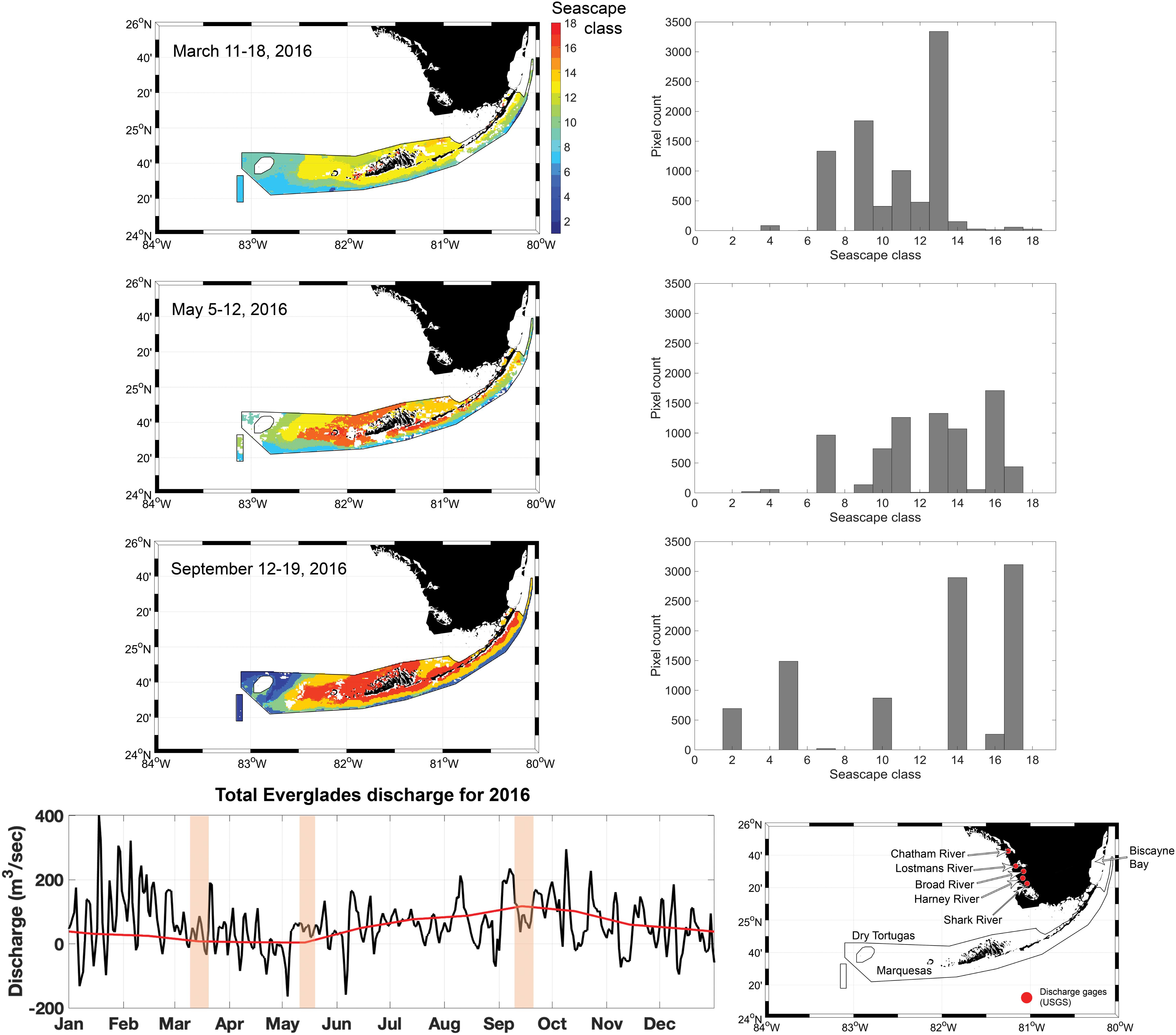
Figure 8. Eight-day composite seascape maps within the FKNMS boundaries only (left) during the three cruise periods (top to bottom). Bar plots show pixel counts of each seascape class extracted from corresponding maps. The time series plot at the bottom shows average daily discharge for 2016 (black line) based on flow data collected at five discharge gages managed by the U.S. Geological Survey (shown in adjacent map). The red line shows the discharge climatology (1997–2018). Shaded bars highlight the sampling period of each cruise.
In May, several classes were present in the FKNMS with comparable areal extent (Figure 8). Over 15% of the Sanctuary was bathed by Warm, Eutrophic, Optically Shallow seascape (class 16), which is largely dominated by diatoms. This class also has a high nFLH signal (∼ 0.2 mW cm–2 μm–1 sr–1; Table 1) indicative of bloom conditions in this region (Hu et al., 2005). Other seascapes with over 10% coverages also showed intermediate to high CDOM concentrations (ag ≈ 0.1–0.3 m–1; Supplementary Figure S3), especially Florida Bay classes (14 and 15), suggesting a strong freshwater influence from the Everglades. Average discharge was slightly higher during this time compared to the previous cruise. Under these conditions optical depth and overall water quality conditions are likely sub-optimal for benthic organisms, with curtailed light availability during this time. Mixed seascape conditions also suggest exposure of benthic habitats to high variability of thermal conditions with possible impacts to metabolic performance of fishes and coral reefs in these areas. For example, a shift in seascapes from Florida Bay Cool to Florida Bay Warm (13 and 14) could lead to a temperature drop of as much as ∼ 5°C.
In September, over 50% of the Sanctuary was bathed by Summer, Nearshore, Optically Shallow (class 17) and Florida Bay Warm (class 14) seascapes, from the Upper Keys south of Biscayne Bay through west of Marquesas Keys toward Dry Tortugas (Figure 8). These are very warm classes almost reaching 29°C and thus some level of thermal stress can be expected in shallow benthic habitats under sustained occupancy of these seascapes. Water quality conditions of these classes could also affect photosynthetic performance of benthic organisms due to high light attenuation by phytoplankton mainly dominated by micro- and nano-phytoplankton size classes (∼ 60–70%). These classes also carry high concentrations of non-algal particles that further attenuate light penetration through the water column (Figure 6). Furthermore, high levels of chl-a, nFLH, non-algal particles and CDOM in seascapes 14 and 17 are consistent with increased Everglades runoff during the 2 weeks prior to the cruise (Figures 6, 8). In deeper waters along the southern edge of the FKNMS, however, seascape conditions were indicative of low phytoplankton concentrations and thus high water clarity conditions. We observed significantly higher dominance of Very Warm, Very Oligotrophic (class 2) and Warm, Oligotrophic (class 5) seascapes not detected during the March or May cruises within the Sanctuary. When these classes occur over coral reefs and seagrasses, light availability may be higher but so is thermal stress with temperatures exceeding 29°C.
Penetration of Florida Bay, Nearshore, and Optically Shallow seascapes (classes 13 through 18) carrying elevated CDOM, non-algal particles and phytoplankton loads over the reef track and the Marquesas Keys likely results from the transfer of waters from Florida Bay and the West Florida Shelf through connecting channels. Outflow of these seascapes into the southern portion of the FKNMS makes benthic habitats particularly sensitive to intermittent sub-optimal water quality conditions. Based on satellite diffuse attenuation coefficient (Kd) and remote sensing reflectance (Rrs) anomalies Barnes et al. (2013, 2014) reported large shifts in water clarity in the Middle and Lower Keys possibly due to discharge from Florida Bay and the West Florida Shelf. Other studies suggest that degradation of seagrass beds and coral reefs in the FKNMS is likely driven by nutrient inputs from these areas, which in turn stimulate phytoplankton growth and thus poor light conditions over the reef track (Hu et al., 2004; Lapointe et al., 2004). However, long-term trends in nutrient concentration in waters bathing these benthic habitats are yet not clear due to observational limitations related to low sampling frequent and spatial coverage. Sediment resuspension and associated turbidity is possibly a major driver of water column light attenuation in the very shallow areas of Florida Bay and West Florida Shelf (Hall et al., 1999; Barnes et al., 2014). Therefore, dominance of lower water clarity seascapes can be expected along the western FKNMS during outflow events of water masses with high concentrations of non-algal particles from the northern portion of the Sanctuary (Stumpf et al., 1999).
Our results demonstrate that the seascape framework can be used to rapidly evaluate seasonal and high-frequency changes in water quality within a marine protected area (MPA) and its surroundings to examine their possible impacts on benthic habitats providing critical ecosystem services. Seascapes can help evaluate the extent to which water quality conditions change over time and space within and around MPAs, investigate why these are changing, and implement effective strategies for conservation and management of living resources based on a coherent, spatially explicit and temporally dynamic, standardized synoptic approach.
Conclusion
Seascapes serve as integrated environmental proxy indicators to examine impacts of various water quality conditions on benthic habitats and species populations, and therefore on fisheries and other relevant ecosystem services. Real-time tracking of seascape occupancy (e.g., shifts or persistence) can inform on the evolution of water quality and thermal properties in critical habitats in support of conservation and management efforts. Seascape data can aid in establishing baseline oceanographic conditions at local to regional scales, including optically shallow areas, and determine how these change over time and space to better gauge the responses of species populations, ecosystem health, and overall biodiversity to environmental change. Seascape observations can also provide insights into dominant phytoplankton groups within water masses of different oceanographic conditions. In this study we found that phytoplankton communities characterized by in situ pigments and bio-optical measurements have a consistent association pattern with seascape classes. Our results indicate that oceanic seascapes are mainly occupied by small phytoplankton taxa such as Synechococcus spp. and Prochlorococcus sp. whereas more coastal seascapes are dominated larger groups like diatoms and dinoflagellates. These observations can help track phytoplankton phenology, ecological connectivity, land-ocean interactions, and areas with transient or persistent exposure to runoff or circulation patterns to guide policy and marine spatial planning more effectively, better protect marine habitats, and sustainably use natural living resources.
Data Availability Statement
All pigment and bio-optical data are available on the NASA SeaWiFS Bio-optical Archive and Storage System (SeaBASS).
Author Contributions
AD contributed to statistical analysis for identifying relationships between seascape classes and phytoplankton communities. FM-K and CK contributed to field data, knowledge on underlying process controlling water quality in the Florida Keys, and ideas on conceptual framework for validation of seascapes. MK provided the seascape classification data for the study region and technical approaches for the seascape validation. All authors contributed to ideas and knowledge on experimental design, methodological approach, and interpretation of results.
Conflict of Interest
The authors declare that the research was conducted in the absence of any commercial or financial relationships that could be construed as a potential conflict of interest.
Acknowledgments
This manuscript is a contribution to the Marine Biodiversity Observation Network (MBON) of the Group on Earth Observations Biodiversity Observation Network. The work was funded under the US National Ocean Partnership Program (NASA, NOAA, U.S. IOOS, BOEM, and ONR) through NASA grant NNX14AP62A [“National Marine Sanctuaries as Sentinel Sites for a Demonstration Marine Biodiversity Observation Network (MBON)”] and Department of the Navy Award NA19NOS0120199 [“Implementing a Marine Biodiversity Observation Network (MBON) in South Florida to Advance Ecosystem-Based Management”]. Additional support was provided by NSF Grant Number 1728913 [“Research Coordination Networks (RCN): Sustained Multidisciplinary Ocean Observations” – the OceanObs RCN]. The manuscript is also a contribution to the Integrated Marine Biosphere Research (IMBeR) project, which is supported by the Scientific Committee on Oceanic Research (SCOR) and Future Earth. Mention of trade names or commercial products does not constitute endorsement or recommendation for use by the US Government. The views expressed in this article are those of the authors and do not necessarily reflect the views or policies of US Government Agencies.
Supplementary Material
The Supplementary Material for this article can be found online at: https://www.frontiersin.org/articles/10.3389/fmars.2020.00575/full#supplementary-material
FIGURE S1 | Hierarchical cluster analysis derived from HPLC pigment ratios calculated as described in section “HPLC Pigment and CHEMTAX Analyses” of the Methods for the March, May, and September 2016 cruises (A–C), respectively). Main clusters are indicated with colors. Binning of the pigment data for CHEMTAX analysis was carried out according to the corresponding colored cluster. Dendrogram labels correspond to station ID’s shown in Figure 1.
FIGURE S2 | Relative abundance of phytoplankton groups derived from CHEMTAX analysis at sampled stations during March, May, and September 2016 cruises (A–C), respectively, and combined data (D). Dendrograms above stack plots are the same as in Figure 3 for reference. Seascape class observed at each station is shown with color bars below stack plots. Station ID’s are as in Figure 1. Dashed rectangles highlight clustering of stations where Mesotrophic and Transition seascapes (classes 10 through 12; Table 1) are dominant classes.
FIGURE S3 | CDOM absorption (ag) at 443 nm measured at sampled sites during the March, May, and September 2016 cruises (A–C), respectively. Bar plot shows average ag(443) in seascape classes 10 through 18 derived from combined data collected the during these cruises. Error bars show standard error.
FIGURE S4 | Similarity matrices showing cophenetic correlation coefficients between dendrogram clusters derived from the second derivative of band-normalized phytoplankton absorption spectra [aphy(λ)/aphy(440)] versus HPLC pigments (A–C) and seascape class (D–F). Absorption-based dendrograms were constructed using different combinations of spectral range and then compared to dendrograms derived from HPLC pigments or seascape class data. Lower and upper limits of spectral ranges are indicated in the Y and X axis, respectively, within 10 nm bins. Left, middle, and right panels correspond to data collected during March, May, and September 2016 cruises, respectively.
Footnotes
References
Aiken, J., Pradhan, Y., Barlow, R., Lavender, S., Poulton, A., Holligan, P., et al. (2009). Phytoplankton pigments and functional types in the Atlantic Ocean: a decadal assessment, 1995–2005. Deep Sea Res. Part II 56, 899–917. doi: 10.1016/j.dsr2.2008.09.017
Alvain, S., Moulin, C., Dandonneau, Y., and Loisel, H. (2008). Seasonal distribution and succession of dominant phytoplankton groups in the global ocean: a satellite view. Glob. Biogeochem. Cycles 22. doi: 10.1029/2007GB003154
Anouar, F., Badran, F., and Thiria, S. (1998). Probabilistic self-organizing map and radial basis function networks. Neurocomputing 20, 83–96. doi: 10.1016/S0925-2312(98)00026-25
Araujo, M. L. V., Mendes, C. R. B., Tavano, V. M., Garcia, C. A. E., and Baringer, M. O. (2017). Contrasting patterns of phytoplankton pigments and chemotaxonomic groups along 30°S in the subtropical South Atlantic Ocean. Deep Sea Res. Part I 120, 112–121. doi: 10.1016/j.dsr.2016.12.004
Barlow, R., Gibberd, M.-J., Lamont, T., Aiken, J., and Holligan, P. (2016). Chemotaxonomic phytoplankton patterns on the eastern boundary of the Atlantic Ocean. Deep Sea Res. Part I 111, 73–78. doi: 10.1016/j.dsr.2016.02.011
Barnes, B. B., Hu, C., Holekamp, K. L., Blonski, S., Spiering, B. A., Palandro, D., et al. (2014). Use of Landsat data to track historical water quality changes in Florida Keys marine environments. Remote Sens. Environ. 140, 485–496. doi: 10.1016/j.rse.2013.09.020
Barnes, B. B., Hu, C., Schaeffer, B. A., Lee, Z., Palandro, D. A., and Lehrter, J. C. (2013). MODIS-derived spatiotemporal water clarity patterns in optically shallow Florida Keys waters: a new approach to remove bottom contamination. Remote Sens. Environ. 134, 377–391. doi: 10.1016/j.rse.2013.03.016
Bidigare, R. R. (1989). “Photosynthetic pigment composition of the brown tide alga: unique chlorophyll and carotenoid derivatives,” in Novel Phytoplankton Blooms, eds E. M. Cosper, V. M. Bricelj, and E. J. Carpenter (Berlin: Springer), 57–75. doi: 10.1007/978-3-642-75280-3_4
Boyce, D. G., Lewis, M. R., and Worm, B. (2010). Global phytoplankton decline over the past century. Nature 466, 591–596. doi: 10.1038/nature09268
Boyd, P. W., and Doney, S. C. (2002). Modelling regional responses by marine pelagic ecosystems to global climate change. Geophys. Res. Lett. 29:53. doi: 10.1029/2001GL014130
Brewin, R. J. W., Sathyendranath, S., Hirata, T., Lavender, S. J., Barciela, R. M., and Hardman-Mountford, N. J. (2010). A three-component model of phytoplankton size class for the Atlantic Ocean. Ecol. Model. 221, 1472–1483. doi: 10.1016/j.ecolmodel.2010.02.014
Bricaud, A., and Stramski, D. (1990). Spectral absorption coefficients of living phytoplankton and nonalgal biogenous matter: a comparison between the Peru upwelling area and the Sargasso Sea. Limnol. Oceanogr. 35, 562–582. doi: 10.4319/lo.1990.35.3.0562
Cannizzaro, J. P., Barnes, B. B., Hu, C., Corcoran, A. A., Hubbard, K. A., Muhlbach, E., et al. (2019). Remote detection of cyanobacteria blooms in an optically shallow subtropical lagoonal estuary using MODIS data. Remote Sens. Environ. 231:111227. doi: 10.1016/j.rse.2019.111227
Catlett, D., and Siegel, D. A. (2018). Phytoplankton pigment communities can be modeled using unique relationships with spectral absorption signatures in a dynamic coastal environment: modeling pigment communities. J. Geophys. Res. Oceans 123, 246–264. doi: 10.1002/2017JC013195
Chase, A., Boss, E., Zaneveld, R., Bricaud, A., Claustre, H., Ras, J., et al. (2013). Decomposition of in situ particulate absorption spectra. Methods Oceanogr. 7, 110–124. doi: 10.1016/j.mio.2014.02.002
Chase, A. P., Boss, E., Cetinić, I., and Slade, W. (2017). Estimation of phytoplankton accessory pigments from hyperspectral reflectance spectra: toward a global algorithm. J. Geophys. Res. Oceans 122, 9725–9743. doi: 10.1002/2017JC012859
Devred, E., Sathyendranath, S., and Platt, T. (2007). Delineation of ecological provinces using ocean colour radiometry. Mar. Ecol. Prog. Ser. 346, 1–13. doi: 10.3354/meps07149
Duffy, J. E., Amaral-Zettler, L. A., Fautin, D. G., Paulay, G., Rynearson, T. A., Sosik, H. M., et al. (2013). Envisioning a marine biodiversity observation network. Bioscience 63, 350–361. doi: 10.1525/bio.2013.63.5.8
El Hourany, R., Abboud-Abi Saab, M., Faour, G., Aumont, O., Crépon, M., and Thiria, S. (2019a). Estimation of secondary phytoplankton pigments from satellite observations using self-organizing maps (SOMs). J. Geophys. Res. Oceans 124, 1357–1378. doi: 10.1029/2018JC014450
El Hourany, R., Abboud-Abi Saab, M., Faour, G., Mejia, C., Crépon, M., and Thiria, S. (2019b). Phytoplankton diversity in the mediterranean sea from satellite data using self-organizing maps. J. Geophys. Res. Oceans 124, 5827–5843. doi: 10.1029/2019JC015131
Falkowski, P., and Kiefer, D. A. (1985). Chlorophyll a fluorescence in phytoplankton: relationship to photosynthesis and biomass. J. Plankton Res. 7, 715–731. doi: 10.1093/plankt/7.5.715
Friedland, K. D., Mouw, C. B., Asch, R. G., Ferreira, A. S. A., Henson, S., Hyde, K. J. W., et al. (2018). Phenology and time series trends of the dominant seasonal phytoplankton bloom across global scales. Glob. Ecol. Biogeogr. 27, 551–569. doi: 10.1111/geb.12717
Game, E. T., Grantham, H. S., Hobday, A. J., Pressey, R. L., Lombard, A. T., Beckley, L. E., et al. (2009). Pelagic protected areas: the missing dimension in ocean conservation. Trends Ecol. Evol. 24, 360–369. doi: 10.1016/j.tree.2009.01.011
Gibb, S. W., Barlow, R. G., Cummings, D. G., Rees, N. W., Trees, C. C., Holligan, P., et al. (2000). Surface phytoplankton pigment distributions in the Atlantic Ocean: an assessment of basin scale variability between 50°N and 50°S. Prog. Oceanogr. 45, 339–368. doi: 10.1016/S0079-6611(00)00007-0
Hales, B., Strutton, P. G., Saraceno, M., Letelier, R., Takahashi, T., Feely, R., et al. (2012). Satellite-based prediction of pCO2 in coastal waters of the eastern North Pacific. Prog. Oceanogr. 103, 1–15. doi: 10.1016/j.pocean.2012.03.001
Hall, M. O., Durako, M. J., Fourqurean, J. W., and Zieman, J. C. (1999). Decadal changes in seagrass distribution and abundance in Florida Bay. Estuaries 22, 445–459. doi: 10.2307/1353210
Hardman-Mountford, N. J., Hirata, T., Richardson, K. A., and Aiken, J. (2008). An objective methodology for the classification of ecological pattern into biomes and provinces for the pelagic ocean. Remote Sens. Environ. 112, 3341–3352. doi: 10.1016/j.rse.2008.02.016
Hays, G., Richardson, A., and Robinson, C. (2005). Climate change and marine plankton. Trends Ecol. Evol. 20, 337–344. doi: 10.1016/j.tree.2005.03.004
Hazen, E. L., Jorgensen, S., Rykaczewski, R. R., Bograd, S. J., Foley, D. G., Jonsen, I. D., et al. (2013). Predicted habitat shifts of Pacific top predators in a changing climate. Nat. Clim. Chang. 3, 234–238. doi: 10.1038/nclimate1686
Higgins, H. W., Wright, S. W., and Schlüter, L. (2011). “Quantitative interpretation of chemotaxonomic pigment data,” in Phytoplankton Pigments, eds S. Roy, C. Llewellyn, E. S. Egeland, and G. Johnsen (Cambridge: Cambridge University Press), 257–313. doi: 10.1017/CBO9780511732263.010
Hirata, T., Hardman-Mountford, N. J., Brewin, R. J. W., Aiken, J., Barlow, R., Suzuki, K., et al. (2011). Synoptic relationships between surface Chlorophyll-a and diagnostic pigments specific to phytoplankton functional types. Biogeosciences 8, 311–327. doi: 10.5194/bg-8-311-2011
Hooker, S. B., Van Heukelem, L., Thomas, C. S., Claustre, H., Ras, J., Barlow, R., et al. (2005). The Second SeaWiFS HPLC Analysis Round-Robin Experiment (SeaHARRE-2). Washington, DC: NASA.
Hu, C., Muller-Karger, F. E., Taylor, C., Carder, K. L., Kelble, C., Johns, E., et al. (2005). Red tide detection and tracing using MODIS fluorescence data: a regional example in SW Florida coastal waters. Remote Sens. Environ. 97, 311–321. doi: 10.1016/j.rse.2005.05.013
Hu, C., Muller-Karger, F. E., Vargo, G. A., Neely, M. B., and Johns, E. (2004). Linkages between coastal runoff and the Florida Keys ecosystem: a study of a dark plume event. Geophys. Res. Lett. 31. doi: 10.1029/2004GL020382
Irwin, A. J., Finkel, Z. V., Müller-Karger, F. E., and Troccoli Ghinaglia, L. (2015). Phytoplankton adapt to changing ocean environments. Proc. Natl. Acad. Sci. U.S.A. 112, 5762–5766. doi: 10.1073/pnas.1414752112
Kavanaugh, M. T., Hales, B., Saraceno, M., Spitz, Y. H., White, A. E., and Letelier, R. M. (2014). Hierarchical and dynamic seascapes: a quantitative framework for scaling pelagic biogeochemistry and ecology. Prog. Oceanogr. 120, 291–304. doi: 10.1016/j.pocean.2013.10.013
Kavanaugh, M. T., Oliver, M. J., Chavez, F. P., Letelier, R. M., Muller-Karger, F. E., and Doney, S. C. (2016). Seascapes as a new vernacular for pelagic ocean monitoring, management and conservation. ICES J. Mar. Sci. 73, 1839–1850. doi: 10.1093/icesjms/fsw086
Kiefer, D. A. (1973). Fluorescence properties of natural phytoplankton populations. Mar. Biol. 22, 263–269. doi: 10.1007/BF00389180
Kishino, M., Takahashi, M., Okami, N., and Ichimura, S. (1985). Estimation of the spectral absorption coefficients of phytoplankton in the sea. Bull. Mar. Sci. 37:9.
Lapointe, B. E., Barile, P. J., and Matzie, W. R. (2004). Anthropogenic nutrient enrichment of seagrass and coral reef communities in the Lower Florida Keys: discrimination of local versus regional nitrogen sources. J. Exp. Mar. Biol. Ecol. 308, 23–58. doi: 10.1016/j.jembe.2004.01.019
Lewison, R., Hobday, A. J., Maxwell, S., Hazen, E., Hartog, J. R., Dunn, D. C., et al. (2015). Dynamic ocean management: Identifying the critical ingredients of dynamic approaches to ocean resource management. Bioscience 65, 486–498. doi: 10.1093/biosci/biv018
Lorenzoni, L., Toro-Farmer, G., Varela, R., Guzman, L., Rojas, J., Montes, E., et al. (2015). Characterization of phytoplankton variability in the Cariaco Basin using spectral absorption, taxonomic and pigment data. Remote Sens. Environ. 167, 259–268. doi: 10.1016/j.rse.2015.05.002
Mackey, M., Mackey, D., Higgins, H., and Wright, S. (1996). CHEMTAX - a program for estimating class abundances from chemical markers: application to HPLC measurements of phytoplankton. Mar. Ecol. Prog. Ser. 144, 265–283. doi: 10.3354/meps144265
McCune, B., Grace, J. B., and Urban, D. L. (2002). Analysis of Ecological Communities. Gleneden Beach, Oregon: MjM Software Design. Available online at: https://trove.nla.gov.au/version/27016941 (accessed May 1, 2019).
Mitchell, G., and Kiefer, D. A. (1988). Chlorophyll a specific absorption and fluorescence excitation spectra for light-limited phytoplankton. Deep Sea Res. 35, 639–663. doi: 10.1016/0198-0149(88)90024-6
Mojica, K. D. A., Poll, W. H., van de Kehoe, M., Huisman, J., Timmermans, K. R., Buma, A. G. J., et al. (2015). Phytoplankton community structure in relation to vertical stratification along a north-south gradient in the Northeast Atlantic Ocean. Limnol. Oceanogr. 60, 1498–1521. doi: 10.1002/lno.10113
Muller-Karger, F. E., Astor, Y. M., Benitez-Nelson, C. R., Buck, K. N., Fanning, K. A., Lorenzoni, L., et al. (2019). The scientific legacy of the CARIACO Ocean time-series program. Annu. Rev. Mar. Sci. 11, 413–437. doi: 10.1146/annurev-marine-010318-095150
Muller-Karger, F. E., Kavanaugh, M. T., Montes, E., Balch, W. M., Breitbart, M., Chavez, F. P., et al. (2014). A framework for a marine biodiversity observing network within changing continental shelf seascapes. Oceanography 27, 18–23. doi: 10.5670/oceanog.2014.56
Mutshinda, C. M., Troccoli-Ghinaglia, L., Finkel, Z. V., Müller-Karger, F. E., and Irwin, A. J. (2013). Environmental control of the dominant phytoplankton in the Cariaco Basin: a hierarchical Bayesian approach. Mar. Biol. Res. 9, 246–260. doi: 10.1080/17451000.2012.731693
Nair, A., Sathyendranath, S., Platt, T., Morales, J., Stuart, V., Forget, M.-H., et al. (2008). Remote sensing of phytoplankton functional types. Remote Sens. Environ. 112, 3366–3375. doi: 10.1016/j.rse.2008.01.021
Nunes, S., Latasa, M., Gasol, J. M., and Estrada, M. (2018). Seasonal and interannual variability of phytoplankton community structure in a Mediterranean coastal site. Mar. Ecol. Prog. Ser. 592, 57–75. doi: 10.3354/meps12493
Oliver, M. J., and Irwin, A. J. (2008). Objective global ocean biogeographic provinces. Geophys. Res. Lett. 35:L15601. doi: 10.1029/2008GL034238
Pinckney, J. L., Benitez-Nelson, C. R., Thunell, R. C., Muller-Karger, F., Lorenzoni, L., Troccoli, L., et al. (2015). Phytoplankton community structure and depth distribution changes in the Cariaco basin between 1996 and 2010. Deep Sea Res. Part I 101, 27–37. doi: 10.1016/j.dsr.2015.03.004
Pinckney, J. L., Richardson, T. L., Millie, D. F., and Paerl, H. W. (2001). Application of photopigment biomarkers for quantifying microalgal community composition and in situ growth rates. Org. Geochem. 32, 585–595. doi: 10.1016/S0146-6380(00)00196-190
Platt, T., and Sathyendranath, S. (1999). Spatial structure of pelagic ecosystem processes in the global ocean. Ecosystems 2, 384–394. doi: 10.1007/s100219900088
Rêve-Lamarche, A.-H., Alvain, S., Racault, M.-F., Dessailly, D., Guiselin, N., Jamet, C., et al. (2017). Estimation of the potential detection of diatom assemblages based on ocean color radiance anomalies in the north sea. Front. Mar. Sci. 4:408. doi: 10.3389/fmars.2017.00408
Reygondeau, G., Longhurst, A., Martinez, E., Beaugrand, G., Antoine, D., and Maury, O. (2013). Dynamic biogeochemical provinces in the global ocean. Glob. Biogeochem. Cycles 27, 1046–1058. doi: 10.1002/gbc.20089
Reynolds, R. A., and Stramski, D. (2019). Optical characterization of marine phytoplankton assemblages within surface waters of the western Arctic Ocean. Limnol. Oceanogr. 64, 2478–2496. doi: 10.1002/lno.11199
Roesler, C. S., Perry, M. J., and Carder, K. L. (1989). Modeling in situ phytoplankton absorption from total absorption spectra in productive inland marine waters: modeling in situ absorption. Limnol. Oceanogr. 34, 1510–1523. doi: 10.4319/lo.1989.34.8.1510
Saraceno, M., Provost, C., and Lebbah, M. (2006). Biophysical regions identification using an artificial neuronal network: a case study in the South Western Atlantic. Adv. Space Res. 37, 793–805. doi: 10.1016/j.asr.2005.11.005
Stumpf, R. P., Frayer, M. L., Durako, M. J., and Brock, J. C. (1999). Variations in water clarity and bottom albedo in Florida Bay from 1985 to 1997. Estuaries 22:431. doi: 10.2307/1353209
Taylor, B. B., Torrecilla, E., Bernhardt, A., Taylor, M. H., Peeken, I., Röttgers, R., et al. (2011). Bio-optical provinces in the eastern Atlantic Ocean and their biogeographical relevance. Biogeosciences 8, 3609–3629. doi: 10.5194/bg-8-3609-2011
Torrecilla, E., Piera, J., and Vilasec, M. (2009). “Derivative analysis of hyperspectral oceanographic data,” in Advances in Geoscience and Remote Sensing, ed. G. Jedlovec (London: IntechOpen), doi: 10.5772/8316
Torrecilla, E., Stramski, D., Reynolds, R. A., Millán-Núñez, E., and Piera, J. (2011). Cluster analysis of hyperspectral optical data for discriminating phytoplankton pigment assemblages in the open ocean. Remote Sens. Environ. 115, 2578–2593. doi: 10.1016/j.rse.2011.05.014
Turner, W., Spector, S., Gardiner, N., Fladeland, M., Sterling, E., and Steininger, M. (2003). Remote sensing for biodiversity science and conservation. Trends Ecol. Evol. 18, 306–314. doi: 10.1016/S0169-5347(03)00070-73
Uitz, J., Claustre, H., Morel, A., and Hooker, S. B. (2006). Vertical distribution of phytoplankton communities in open ocean: an assessment based on surface chlorophyll. J. Geophys. Res. 111. doi: 10.1029/2005JC003207
Ulrich, T. (2020). Ternary Plots. Available online at: https://www.mathworks.com/matlabcentral/fileexchange/7210-ternary-plots (accessed May 16, 2020).
Vaillancourt, R. D., Lance, V. P., and Marra, J. F. (2018). Phytoplankton chemotaxonomy within contiguous optical layers across the western North Atlantic Ocean and its relationship to environmental parameters. Deep Sea Res. Part I 139, 14–26. doi: 10.1016/j.dsr.2018.05.007
Van Heukelem, L., and Thomas, C. S. (2001). Computer-assisted high-performance liquid chromatography method development with applications to the isolation and analysis of phytoplankton pigments. J. Chromatogr. A 910, 31–49. doi: 10.1016/S0378-4347(00)00603-604
Vidussi, F., Claustre, H., Manca, B. B., Luchetta, A., and Marty, J.-C. (2001). Phytoplankton pigment distribution in relation to upper thermocline circulation in the eastern Mediterranean Sea during winter. J. Geophys. Res. Oceans 106, 19939–19956. doi: 10.1029/1999JC000308
Ward, J. H. (1963). Hierarchical grouping to optimize an objective function. J. Am. Stat. Assoc. 58, 236–244. doi: 10.1080/01621459.1963.10500845
Werdell, P. J., Roesler, C. S., and Goes, J. I. (2014). Discrimination of phytoplankton functional groups using an ocean reflectance inversion model. Appl. Opt. 53, 4833–4849. doi: 10.1364/AO.53.004833
Wright, S., Thomas, D., Marchant, H., Higgins, H., Mackey, M., and Mackey, D. (1996). Analysis of phytoplankton of the Australian sector of the Southern Ocean: comparisons of microscopy and size frequency data with interpretations of pigment HPLC data using the “CHEMTAX” matrix factorisation program. Mar. Ecol. Prog. Ser. 144, 285–298. doi: 10.3354/meps144285
Wright, S. W., Ishikawa, A., Marchant, H. J., Davidson, A. T., van den Enden, R. L., and Nash, G. V. (2009). Composition and significance of picophytoplankton in Antarctic waters. Polar Biol. 32, 797–808. doi: 10.1007/s00300-009-0582-589
Xi, H., Losa, S. N., Mangin, A., Soppa, M. A., Garnesson, P., Demaria, J., et al. (2020). Global retrieval of phytoplankton functional types based on empirical orthogonal functions using CMEMS GlobColour merged products and further extension to OLCI data. Remote Sens. Environ. 240:111704. doi: 10.1016/j.rse.2020.111704
Xing, X.-G., Zhao, D.-Z., Liu, Y.-G., Yang, J.-H., Xiu, P., and Wang, L. (2007). An overview of remote sensing of chlorophyll fluorescence. Ocean Sci. J. 42, 49–59. doi: 10.1007/BF03020910
Zhang, J.-Z. (2000). Shipboard automated determination of trace concentrations of nitrite and nitrate in oligotrophic water by gas-segmented continuous flow analysis with a liquid waveguide capillary flow cell. Deep Sea Res. Part I 47, 1157–1171. doi: 10.1016/S0967-0637(99)00085-80
Zhang, J.-Z., and Berberian, G. A. (1997). Determination of Dissolved Silicate in Estuarine and Coastal Waters by Gas Segmented Continuous Flow Colorimetric Analysis. EPA Method 366.0. National Exposure Research Laboratory Office of Research and Development. Cincinnati, OH: U.S. Environmental Protection Agency.
Zhang, J.-Z., Fischer, C. J., and Ortner, P. B. (2000). Continuous flow analysis of phosphate in natural waters using hydrazine as a reductant. Intern. J. Environ. Anal. Chem. 80, 61–73. doi: 10.1080/03067310108044386
Zhang, J.-Z., Ortner, P. B., Fischer, C. J., and Moore, L. D. (1997). Determination of Ammonia in Estuarine and Coastal Waters by Gas Segmented Continuous Flow Colorimetric Analysis. EPA Method 349.0. National Exposure Research Laboratory Office of Research and Development. Cincinnati, OH: U.S. Environmental Protection Agency.
Keywords: Marine Biodiversity Observation Network, Florida Keys National Marine Sanctuary, biogeographic seascapes, phytoplankton functional types, phytoplankton pigment analysis, HPLC, CHEMTAX, bio-optics
Citation: Montes E, Djurhuus A, Muller-Karger FE, Otis D, Kelble CR and Kavanaugh MT (2020) Dynamic Satellite Seascapes as a Biogeographic Framework for Understanding Phytoplankton Assemblages in the Florida Keys National Marine Sanctuary, United States. Front. Mar. Sci. 7:575. doi: 10.3389/fmars.2020.00575
Received: 18 December 2019; Accepted: 22 June 2020;
Published: 15 July 2020.
Edited by:
Angel Borja, Technological Center Expert in Marine and Food Innovation (AZTI), SpainReviewed by:
Tomonori Isada, Hokkaido University, JapanGabriel Navarro, Institute of Marine Sciences of Andalusia (ICMAN), Spain
Copyright © 2020 Montes, Djurhuus, Muller-Karger, Otis, Kelble and Kavanaugh. This is an open-access article distributed under the terms of the Creative Commons Attribution License (CC BY). The use, distribution or reproduction in other forums is permitted, provided the original author(s) and the copyright owner(s) are credited and that the original publication in this journal is cited, in accordance with accepted academic practice. No use, distribution or reproduction is permitted which does not comply with these terms.
*Correspondence: Enrique Montes, emontesh@usf.edu