Most eastern boundary upwelling regions represent thermal refugia in the age of climate change

Introduction

The four major Eastern Boundary Upwelling Systems (EBUS) - Humboldt, Benguela, California, and Iberian/Canary - are characterized by a narrow coastal band (~50–150 km) of surface temperatures that are cooler than temperatures offshore (Bakun and Parrish, 1982; Chavez and Messié, 2009). This is caused by wind-driven coastal upwelling that brings deep, cold water to the surface at the coast. Cool, nutrient-rich upwelled waters fuel large phytoplankton blooms that sustain the rich marine ecosystems of EBUS (Kämpf and Chapman, 2016), including 20% of world fisheries catch (Pauly and Christensen, 1995; Bindoff et al., 2019) and high biodiversity of upper trophic level species (Chavez and Messié, 2009; Watermeyer et al., 2020]. Furthermore, the cool coastal sea surface temperature (SST) footprint is important to adjacent terrestrial ecosystems in driving low clouds (fog), low temperature, and high humidity (Johnstone and Dawson, 2010) that are favorable to forested and agricultural areas (Black et al., 2014). Overall, EBUS provide services to ~80 million people (García-Reyes et al., 2015). On a global scale, the cool EBUS SST footprint affects climate through air-sea interactions (Large and Danabasoglu, 2006; Curchitser et al., 2011; Bakun et al., 2015), as well as CO₂ outgassing (as upwelled water is high in CO₂ content) and capture (through enhanced primary productivity) (Mackas et al., 2006; Ikawa et al., 2013; Brady et al., 2019).

Changes in the cold footprint of upwelling have not been studied extensively as have changes in temperatures along EBUS, although they are clearly related. For example, Santora et al. (2020) quantified the upwelling footprint as the coastal area below a temperature threshold associated with upwelled water, calling it the habitat compression index (HCI). Impacts of warm conditions along EBUS are well documented, for example, during El Niño events along the Pacific EBUS (Chavez et al., 2002; Escribano et al., 2004; Jacox et al., 2016; Diaz-Astudillo et al., 2022), or a marine heatwave (MHW) in the Northeast Pacific in 2014–2016 (Gentemann et al., 2017; Santora et al., 2020); both types of events caused large negative consequences for coastal socio-ecological systems. In the California, variability in the HCI has been associated with changes in zooplankton and forage indices (Schroeder et al., 2022), as well as the risk of humpback whale entanglement in fishing gear due to reduction of cold favorable habitat, which leads to redistribution and overlap of whale prey into crab fishing grounds (Santora et al., 2020). The HCI has demonstrated that changes in upwelling footprint is a good indicator of suitable habitat.

Anthropogenic global climate change is impacting EBUS similarly to other oceanic regions by increasing global ocean temperatures (Cooley et al., 2022; Bograd et al., 2023), stratification (Bakun et al., 2015; Li et al., 2020), and frequency of extreme events such as MHWs (Gentemann et al., 2017; Varela et al., 2021; Izquierdo et al., 2022; Thoral et al., 2022). On the other hand, upwelling-favorable winds are predicted to strengthen in poleward regions of EBUS (Sydeman et al., 2014; Bakun et al., 2015; Rykaczewski et al., 2015; Wang et al., 2015; Abrahams et al., 2021; Bograd et al., 2023), potentially counteracting increasing temperature trends. However, how temperatures in coastal upwelling regions are and will respond to these counteracting drivers has been a subject of debate, with unclear or contradicting trends (Bograd et al., 2023) depending on dataset, period of study, and spatial scale (Sydeman et al., 2014; Bakun et al., 2015; García-Reyes et al., 2015). Few studies have examined SST trends at the spatial scales at which coastal upwelling occurs. Varela et al. (2018) and Seabra et al. (2019) showed that decadal trends in SST along EBUS have changed little, or even cooled, at nearshore locations (within ~50 km) due to the cooling effects of upwelling. For these reasons, EBUS have been hypothesized to be “thermal refugia” from global warming (Bakun et al., 2015; Hu and Guillemin, 2016; Lourenço et al., 2016; Barceló et al., 2018; Varela et al., 2018; Lourenço et al., 2020), but observed regional and seasonal changes in the spatial extent of the surface expression (i.e., “footprint”) of coastal upwelling has yet to be investigated.

A general question of interest is, therefore: as global ocean temperatures rise and marine heatwaves become more frequent (Bindoff et al., 2019), are the upwelling-derived cool-water habitats in EBUS coastal areas changing in a manner that may be detrimental to marine life and coastal societies? This question has yet to be asked across all EBUS. In particular, trends in the upwelling footprint would depend on the relative importance and rate of change of different mechanisms driving temperature change in different regions (see review in Bograd et al., 2023 and in the IPCC’s Cooley et al., 2022). In this study, we address this question by investigating changes in spatial extent of cool SST footprints in EBUS using high-resolution observations collected over the last two decades. We test the null hypothesis of no significant change (expansion or contraction) in the cool-water SST footprint over time, consistent with the concept that EBUS coastal habitat represents thermal refugia to global warming due to the effects of upwelling.

Data & methods

In this study we used an area of 300 km from shore (approximately the extent of national exclusive economic zones (EEZ); see Figures 1, 2) along the EBUS to fully capture variability in the SST associated with upwelling coastal process. This occurs mostly in a narrow band of ~30 km from shore, corresponding to the Rossby radius of deformation (Allen, 1973; Carr and Kearns, 2003), but the cooler SST upwelled can extend to 150 km or more due to offshore transport, especially downstream of upwelling centers like promontories or capes (Chavez and Messié, 2009; Hutchings et al., 2009). These 300-km subregions are embedded in the equatorward eastern boundary currents that occur year-round and can extend hundreds of kilometers offshore (Thiel et al., 2007; Checkley and Barth, 2009; Mason et al., 2011). We selected three subregions within each EBUS (Figure 1, Table 1) based on subregions identified in the literature as dynamically coherent (Tarazona and Arntz, 2001; Thiel et al., 2007; Arístegui et al., 2009; Checkley and Barth, 2009; Hutchings et al., 2009). The subregions were identified by their distinctive seasonality and magnitude in upwelling-favorable winds and sea temperature, with equatorial subregions exhibiting larger temperatures and year-round winds, and poleward subregions with lower temperatures and stronger seasonality in winds. Central subregions in most EBUS exhibit a strong center of seasonal upwelling.

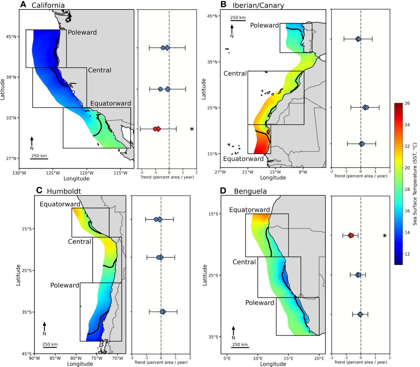
Figure 1 Mean SST (2002-2022, MURSST) in the four major EBUS ((A) California, (B) Iberian/Canary, (C) Humboldt, (D) Benguela), within an area extending 300 km from the shore. Selected subregions within each EBUS are delineated. The black line delimits the threshold SST_T for each subregion that identifies the cool SST footprint. To the right of each map are the trends in annual SST footprint from the GLS model (diamond) and the GLM (circle) for each subregion represented as the percent of the total area per year. Statistically significant trends, based on the two-tail Monte Carlo test, are colored in red and denoted with an asterisk (See Table 1). 95% confidence intervals are shown from the GLS model and indicated by black lines.

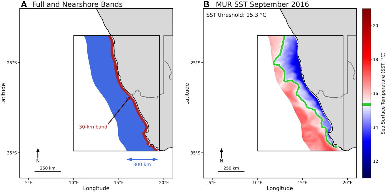
Figure 2 (A) Map of the poleward Benguela subregion illustrating the method of study area delineation. Subregion broad boundaries are shown as a black box, the total area of study is delimited by the ‘blue’ area from the coast to 300 km offshore (this area represents 100% of the possible area of the SST footprint), and the 30-km ‘red’ coastal band is where upwelling occurs and where the SST threshold (SST_T) was calculated as the mean SST within it. (B) Cool SST footprint for September 2016, with color representing monthly SST and the green contour line indicating the subregion SST threshold (SST_T = 15.6°C); the portion of the total area with temperature below the SST_T (green line) is defined as the SST footprint for this month.

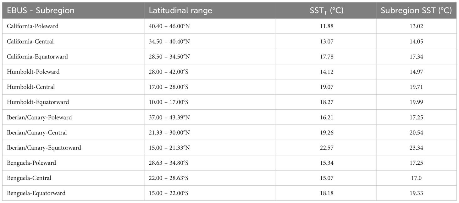
Table 1 Latitudinal range, SST threshold (SST_T) for each subregion (defined mean SST of the coastal band within 30 km from shore for each EBUS), and for comparison, the entire subregion mean SST (from shore to 300 km away from the coast).

We used Multi-scale Ultra-high Resolution (MUR) SST V4.1 data (JPL Mur MEaSUREs Project, 2015; Chin et al., 2017) for a 20-year period (June 1, 2002 to May 31, 2022). MUR SST data are gap-free at daily temporal scales and have a spatial resolution of 1x1 km, which is ideal for this analysis; the fine spatial resolution can most accurately capture the SST footprint extension and its changes. We aggregated the SST data monthly to increase the signal to noise ratio, as we were interested in interannual and longer time scale changes. Another advantage of using MUR SST, despite its relatively short temporal reach, was that it is available worldwide, allowing a comparison across EBUS in recent times. Subregions of SST were then delimited (masked) by the latitudinal range shown in Table S1, the coast, and a longitudinal line 300 km away from the shore. This masked area (colored in Figures 1, 2) constituted the 100% of the area for each subregion.

Inspired by the HCI Index definition from Santora et al. (2020), we defined an indicator of the EBUS cool SST footprint: an area with SST below a given threshold proxying a coastal cool habitat associated with upwelling and mixing of cool and nutrient-rich waters, and therefore biological productivity (Schroeder et al., 2022). This threshold (SST_T) was calculated as the long-term mean SST value of the 30-km coastal band within each subregion (Table 1, red band in Figure 2A) where coastal upwelling occurs. The SST_T used in this research might differ from one more specifically derived based on local upwelling measurements that factor in wind stress or nutrient content, but this one-size-fits-all definition is an objective way to compare SST footprint variability for all subregions, and it was necessary given the heterogeneity in coastal upwelling among and within EBUS. Coastal upwelling shows heterogeneity in phenology, magnitude, and sign of winds and SST through the year (Figure 3) (Bakun and Nelson, 1991; Carr and Kearns, 2003; Escribano and Schneider, 2007; Bograd et al., 2009). However, we used the same subregional threshold SST_T value for the entire subregion, as it is representative of the local upwelling along the subregion coast.

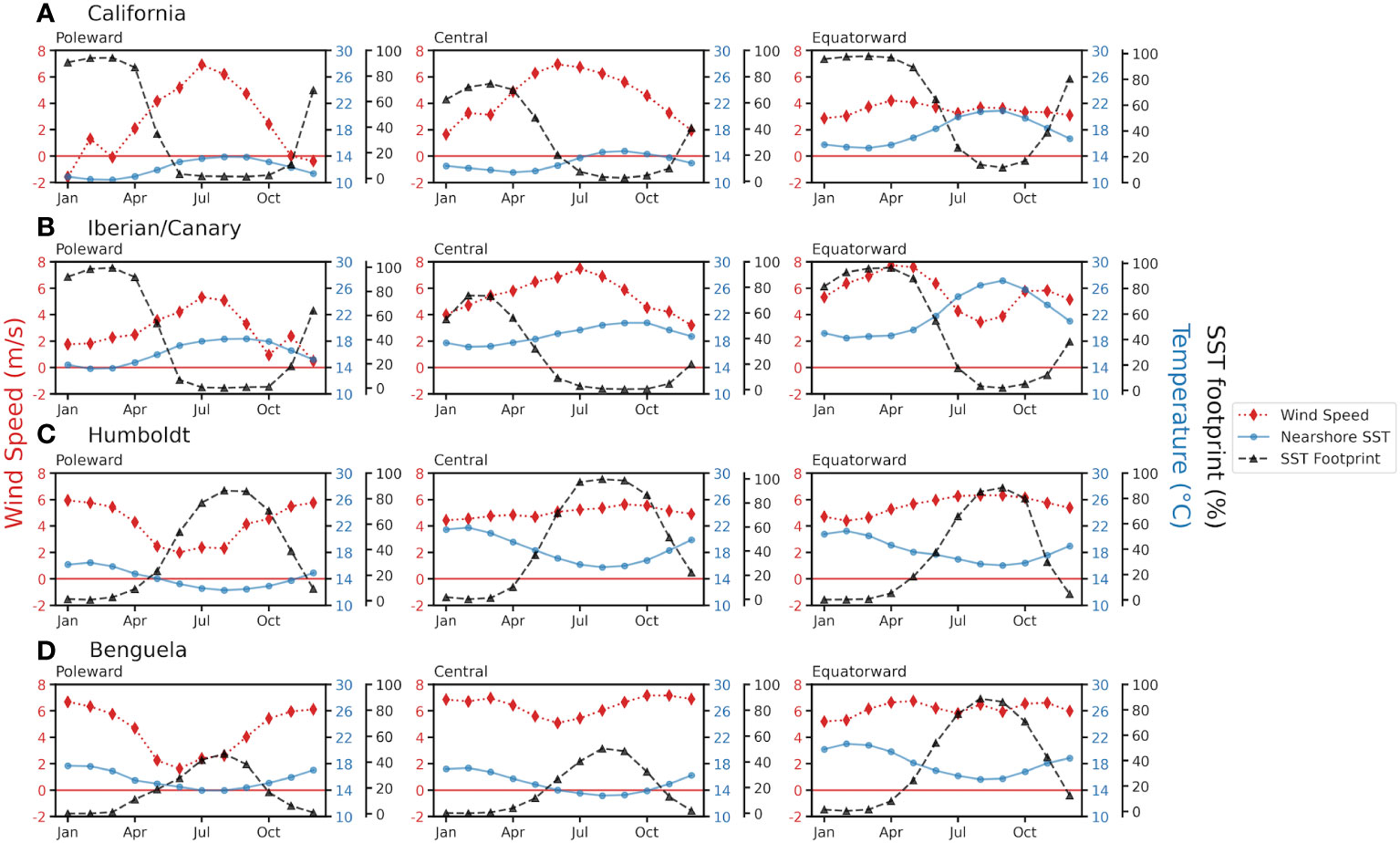
Figure 3 Seasonal cycle of upwelling-favorable meridional wind speed (red diamonds: ERA5 data), SST from the coastal 30-km band (blue dots: MURSST), and cool SST footprint percentage (black triangles; MURSST). Values were based on monthly means for the period 2002-2022, for (A) California, (B) Iberian/Canary, (C) Humboldt, and (D) Benguela EBUS.

The monthly cool SST footprint extension was then calculated as the number of 1x1-km pixels in a given subregion that were below its threshold SST_T (see Figure 2B), and was expressed as a percent of the subregion area (masked) to standardize it. Because the threshold SST_T was based on the SST of the cool 30-km coastal band, the total subregion area was seldom below that value; however, winter temperatures, not necessarily associated with upwelling but not distinguishable from them, could be below the threshold SST_T. Finally, we calculated seasonal and annual averages of the SST footprint. The annual average spanned winter to fall for both hemispheres, covering an entire upwelling season. Winter was defined as December to February for the northern hemisphere and June to August for the southern hemisphere, and so on.

We tested our hypothesis through two methods. First, we used a generalized least square model (GLS) to calculate linear trends for the subregions within each EBUS. To build the GLS, the subregion’s annual SST footprint time series acts as the response variable, year as the time covariate, and EBUS and subregions as categorical values (See supplementary material). Following the methodology laid out by Zuur et al. (2009), the GLS included a weight parameter to help control for heteroskedasticity in the residuals. For this model, a constant variance function was used in which each EBUS was allowed to vary independently. The GLS also included a correlation term that corrected for the non-independence of the residuals, necessary given the relatively short span of the time series. A first order autoregressive structure was fit to the residuals of the model with year as the continuous covariate, and the significance is represented in the results by the confidence intervals. This method allowed us to estimate the linear trends with larger statistical power by increasing the degrees of freedom when combining data together from all subregions. The second approach used generalized linear models (GLM) to individually calculate the trend for each EBUS/subregion time series, and therefore had fewer degrees of freedom given by the length of each time series. These GLMs had a similar formula as the GLS, with percent of the area below SST_T as the response variable and year as a continuous covariate. For the GLM trends a two-tail Monte-Carlo test was used to calculate p-values from a randomized set of similarly distributed data to avoid overestimating statistical significance (p < 0.025 for the two-tail test) due to autocorrelation and length of time series. Both model methods provide similar information, but have different statistical capabilities and we consider them complementary to address the length of the time series and the large interannual variability in some regions. Furthermore, each subregion is large enough to be considered independent from each other (given the smaller Rossby radius of deformation (Huyer, 1983) and the offshore extent of upwelling compared to the distance to the next subregion), therefore, we are not concerned with inflation of p-values by the number of linear regressions calculated.

To investigate changes in the timing of the SST footprint, we calculated linear trends in seasonal means in each subregion’s footprint. Seasonal means were chosen over monthly to avoid over-calculating trends on data that did not necessarily show large changes month to month. In addition, we calculated linear trends of seasonal SST within each EBUS to further describe the spatial distribution of cool SST footprint changes. We used the GLM and Monte-Carlo tests to calculate trends and p-values for these time series. The Python and R code used to generate the indices and analyze the data can be found in a Github repository [https://github.com/farallon-institute/Garcia-Reyes_etal_2023_EBUSFootprint].

Additionally, to illustrate the seasonality of upwelling-favorable wind and SST, we used the monthly seasonality of SST in the 30-km coastal bands and the meridional wind (V) over each EBUS subregion (Figure 3). Meridional wind speed (m/s) was extracted from the ERA5 dataset (Hersbach et al., 2020) for the period 2002–2022. Wind data were provided at 10 m over the sea surface with an hourly temporal resolution and a 31-km spatial resolution. SST was extracted from MUR SST for the same period.

Results

The extent of cool SST footprints in all EBUS subregions show differences in timing and magnitude through their seasonal cycles (Figure 3), with magnitudes varying from 0% to 40–100% (area below the threshold SST_T). The largest cool footprints occur between February and April in the northern hemisphere, and between July and September in the southern hemisphere. The meridional wind and SST seasonalities shown in Figure 3 are consistent with those reported in the literature (Shannon, 2001; Carr and Kearns, 2003; Chavez and Messié, 2009; Montecino and Lange, 2009), but note that the peaks of the SST footprint do not occur simultaneously with the peaks in meridional wind speed (upwelling-favorable) in most subregions (Figure 3). The difference in peak timing indicates that the strong seasonality in temperature due to the solar cycle dominates the timing of the coastal SST annual cycle, rather than upwelling-induced cooling, independently of the cooler SST magnitudes at the coast due to upwelling. In winter, temperatures are below the mean SST threshold, and the SST footprint is large. This is not necessarily due to upwelling (although in equatorial subregions upwelling occurs year-round), but SST values are below those typical of the upwelling season anyway, so they still represent a cool habitat.

The seasonality of the SST footprint unfolds, in general, as follows. During the peak of upwelling-favorable winds, nearshore waters are cooler than offshore. As summer unfolds, the SST footprint contracts, even if upwelling-favorable winds are still present, as deep cool water no longer reaches the surface due to the increasing stratification of the water column caused by the seasonal warming of upper layers of the ocean (Jacox and Edwards, 2011). The poleward Benguela subregion shows the narrowest SST footprint due to the warm influence of the portion of the Agulhas Current that enters the South Atlantic as mesoscale eddies (Hutchings et al., 2009), which leads to a strong cross-shore SST gradient year-round (Figure 1D). In any season, SST footprints can contract for other reasons, such as the occurrence of a marine heatwave, as occurred in 2014–2016 in the California EBUS (Figure S1) (Gentemann et al., 2017).

Linear trends for the annual SST footprint show similar results for the GLS and GLM (Table 2, Figure 1), with no significant trends for 10 of 12 EBUS subregions (p < 0.025 in the two-tail Monte Carlo test in the GLM or p < 0.05 in the GLS); the exceptions are the equatorward Benguela and California subregions, which show a contraction of their annual SST footprints. The equatorward California subregion shows a significant negative large trend in the GLM, but not in the GLS due to the autocorrelation and large interannual variability of the time series (Figure S1). The central California subregion shows a significant negative trend in the GLM, but the Monte Carlo test removes the significance and the trend is small and largely not significant in the GLS (Figure 1) due to autocorrelation and large interannual variability. It is worth noting that despite the lack of statistical significance (p > 0.025 on the Monte Carlo test), trends in other subregions show negative trends of significant magnitude, like central and poleward California in the GLM, and a positive trend in central Iberian/Canary in both models.

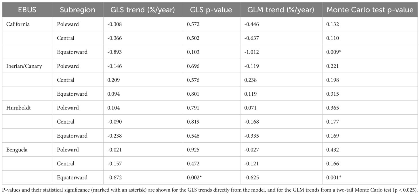
Table 2 Linear trends of annual SST footprint area in %/year for generalized least squared (GLS) model and generalized linear model (GLM).

Seasonal linear trends in SST footprints for each EBUS subregion from the GLM are shown in Figure 4 and Table S1, while the time series are plotted in Figure S2. Trends vary in magnitude, and in some subregions in sign, across seasons. Humboldt and Iberian/Canary show no significant trends in any season (based on the Monte Carlo test), although they show not significant trend in all seasons, especially a positive trend in the fall in central Iberian/Canary and negatives ones in winter and summer in central Humboldt. The Benguela EBUS shows negative trends in winter (significant only in the equatorward subregion), and is more neutral in other seasons for the poleward and central subregions, although the equatorward subregion also shows a negative trend in spring. The California EBUS exhibits the largest negative trends among EBUS, in both its central and equatorward subregions. In the fall, all subregions show contracting (negative) trends in the Monte Carlo test, with the equatorward subregion having the largest trend, and the poleward the smallest. Central and equatorward California regions also show significant negative (contracting) trends in the summer, again, with the equatorward subregion exhibiting the largest negative trend, and the largest interannual variability in all seasons. It is worth noting that the central California spring season has a very small positive trend, the only one in this EBUS for any season.

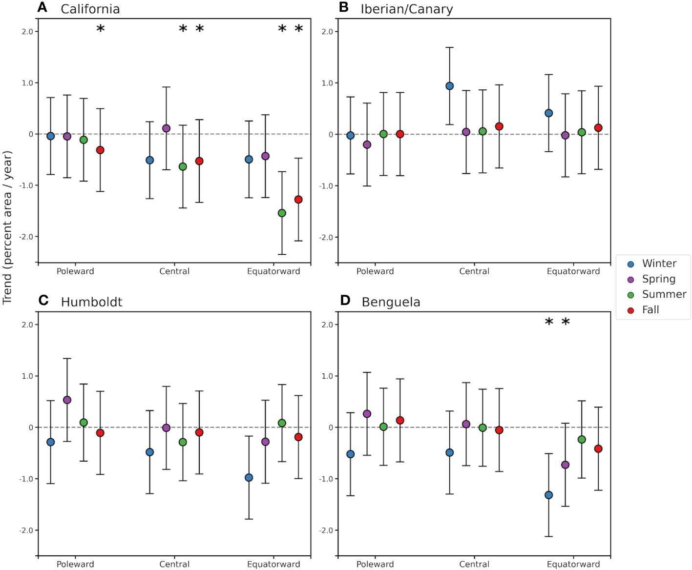
Figure 4 Linear trends of seasonal means of SST footprint (%/year) for each EBUS subregion with 95% confidence intervals from the GLM. Colors indicate seasons; winter is defined as December to February for the northern hemisphere and June to August for the southern hemisphere. Significant trends (p < 0.025 based on two-tail Monte Carlo test) are represented with an asterisk, and confidence intervals are based on the linear regression model. (A) California, (B) Iberian/Canary, (C) Humboldt, and (D) Benguela EBUS.

Seasonal SST trends show narrow coastal regions of decreased temperatures in the central and poleward Benguela, Humboldt, and central Canary subregions, and warming trends in equatorward Benguela and California EBUS (Figures S3–S6). While the trends in most areas were not statistically significant (p>0.05, significance directly from the linear trend calculation at each grid point), the Iberian-Canary and Humboldt EBUS had a mix of small negative and positive trends offshore of the coastal band, while the Benguela and California EBUS had more ubiquitous warming trends, except during the spring season, which were negative. Any negative trend in the EBUS areas is opposed to the warming global SST trends (see Table S2 for global and hemispheric SST trend magnitudes), however, EBUS warming trends, when significant, can be larger than global or hemispherical trends by up to an order of magnitude. For example, the central and equatorward California subregions in the fall and the equatorial Benguela subregions in winter show large patches of significant warming up to 1°C/decade (from 2002 to 2022), while the global SST trend is 0.14°C/decade and the trend for the northern hemisphere is 0.21°C/decade (See Table S2) change into (NOAA Climate at a Glance). Note, however, that SST trends in Figures S3–S6 are representative of the change in temperatures in the region, but their magnitudes are based on pixels of 1 km x 1 km, as per the resolution of the data; smaller trends (and with different statistical significance) would be obtained if spatial averages were considered (as done for global or California EBUS scale analysis).

Discussion

In this paper, we quantify the changes in the coastal cool SST footprint that characterize EBUS. We test if 20-year linear trends in the extension of these footprints are contracting at annual and seasonal scales across EBUS (Table 3). We found that, taken into account the autocorrelation and variability of the time series, 10 out of 12 EBUS subregions support the hypothesis that the extension of the footprint, on annual scales, has not contracted in the last 20 years, despite the continued warming of the global oceans (Fox-Kemper, 2021). This result is in agreement with the idea that EBUS could be considered thermal refugia, and consistent with results from Seabra et al. (2019) showing that coastal areas in EBUS are responding differently to global warming, mostly warming at lower rates than offshore areas. Two subregions, equatorward California and Benguela, however, exhibit a contraction of their annual SST footprint in the period of study, with the former being the largest trend across all subregions. The large interannual variability in the equatorward California, plus the autocorrelation in the time series, removes the statistical significance in the trend in the GLS model, however, as we discuss later, diverging seasonal trends play an important role. Although not significant, the equatorward Humboldt subregion exhibits a contracting trend (negative), but on the contrary, equatorward Iberian/Canary shows an expanding trend. Interestingly, despite the lack of statistical significance, there is a pattern in the trends in which the equatorward regions exhibit the largest contraction trends (negative) and the poleward the smallest or zero (Figure 1), except in the Iberian/Canary EBUS.

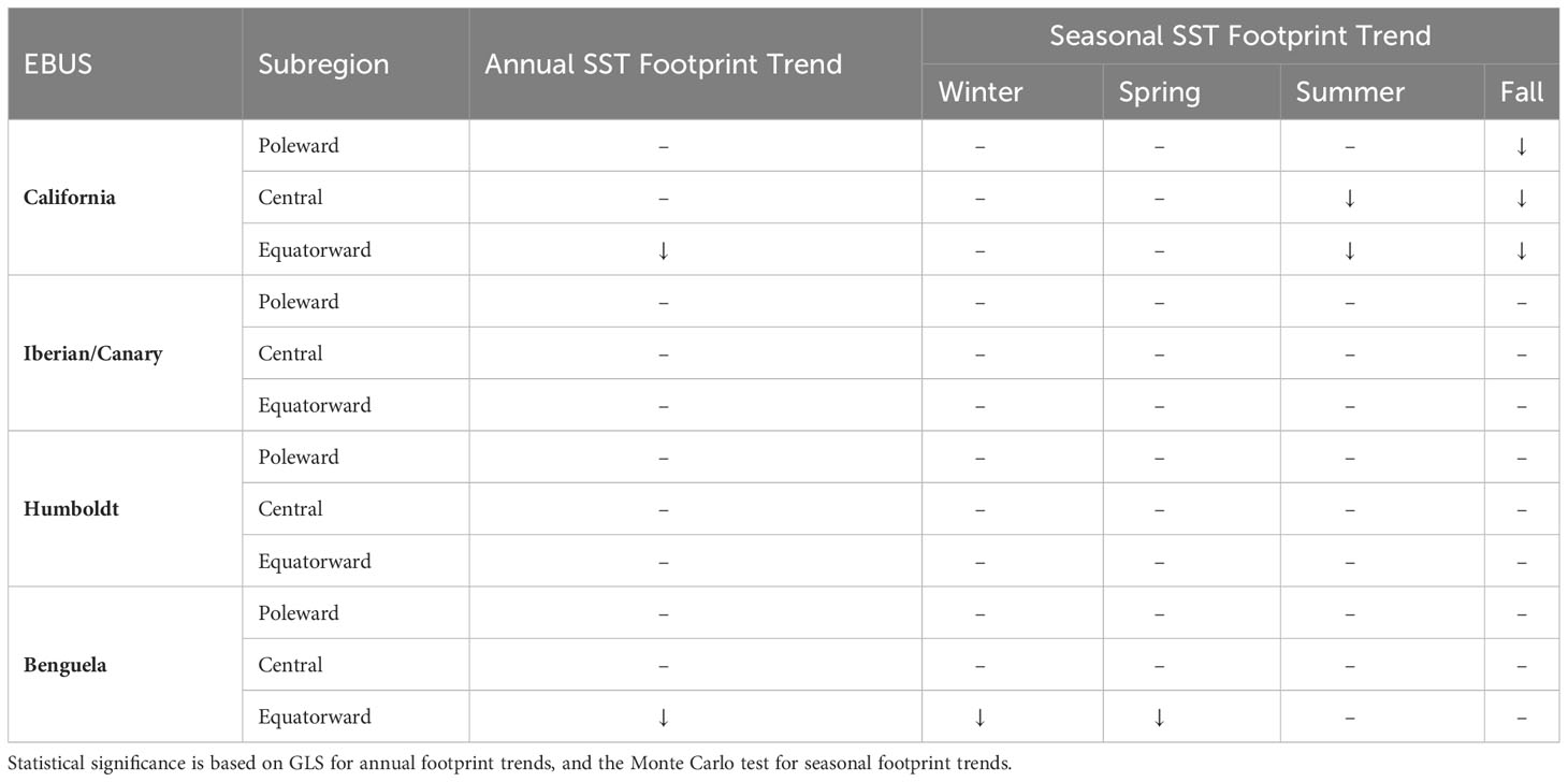
Table 3 Were used in. Summary of locations and timing of statistically significant trends in the annual and seasonal cool SST footprint (downward arrow: contraction; upward arrow: expansion).

This latitudinal pattern appears to be consistent with the weakening of upwelling, stronger water column stratification, and warmer temperatures in equatorward regions of EBUS predicted under climate change (Bakun et al., 2015; García-Reyes et al., 2015; Rykaczewski et al., 2015; Wang et al., 2015). The reported strengthening of upwelling-favorable winds in recent decades (Sydeman et al., 2014; Varela et al., 2015; Bindoff et al., 2019; Bograd et al., 2023) and predicted under climate change (Bakun, 1990; Rykaczewski et al., 2015; Wang et al., 2015; Bindoff et al., 2019) is not reflected in an expansion of cool SST footprints, although we observe cooling of coastal waters during the study period across EBUS, except California. It is possible, however, that the lack of expansion is caused by the increasing offshore temperatures (Seabra et al., 2019; Fox-Kemper, 2021), pressing on EBUS coastal footprints.

The lack of contraction of annual SST footprints in most EBUS, however, is encouraging, and it is supported from previous studies showing that in coastal areas of the EBUS, upwelling appears to mitigate or counteract the global ocean warming trend observed elsewhere (Santos et al., 2012; Varela et al., 2018; Seabra et al., 2019; Abrahams et al., 2021; Izquierdo et al., 2022). This suggests that, for the period 2002–2022, local processes like coastal upwelling, winter mixing, and longwave cooling have been strong or stable enough to counteract global warming trends and/or regional climate processes that drive low-frequency variability in EBUS conditions (Bonino et al., 2019; Marin et al., 2021). Notably, for the period of this study, the Humboldt EBUS does not show the reported cooling (corresponding to contraction of the SST footprint) trends observed in other datasets with longer time series (Varela et al., 2018; Seabra et al., 2019; Abrahams et al., 2021), while California shows significant contraction and warming at seasonal scales (see below).

Given the short length of the time series in climate time-scales, the observed trends might not be a reflection of climate change only, but also of basin-scale decadal climate oscillations. This is particularly the case of the Iberian/Canary poleward subregion, which exhibits opposite trends (positive, expansion) in annual SST footprint to other EBUS, although not statistically significant, and the California EBUS where the largest variability is observed (Figures S1, S2). However, the Iberian/Canary trends are consistent with previous results showing trends in upwelling-associated indicators divergent from other EBUS (Sydeman et al., 2014; Varela et al., 2015; Abrahams et al., 2021; Bograd et al., 2023). These differences among EBUS trends (in sign and magnitude) are addressed in a modeling study by Bonino et al. (2019) which shows that different regional mechanisms drive SST variability in each basin: California and Humboldt systems respond largely and synchronously to El Niño variability, Benguela responds to long-term anthropogenic climate change, and Iberian/Canary responds to North Atlantic multi-decadal variability. While results presented here are mostly consistent with Bonino et al. (2019), (seen for example in the large interannual variability in the California EBUS, associated with El Niño in 2016 and the preceding large marine heatwave in 2014–2015 that impacted the trends and their significance), in the poleward Humboldt cooling has been associated with strengthening upwelling-favorable winds and regional cooling temperatures (Varela et al., 2015; Abrahams et al., 2021), rather than the large interannual variability associated with El Niño observed in the equatorial subregion and in the California EBUS. As global ocean warming is expected to continue (Fox-Kemper, 2021), it is likely, however, that warming trends might become significant in all subregions, despite upwelling-favorable wind trends or regional multi-decadal oscillations, due to increased offshore SST, increased ocean temperature at depth, and increased stratification that limits the efficacy of upwelling to bring deeper, cooler waters to the surface (Bakun et al., 2015; Li et al., 2020).

Since coastal upwelling is mostly a seasonal process in EBUS, we further investigate changes in SST footprints by calculating linear trends of seasonal means of SST footprint for each EBUS subregion (Figure 4, Table S1) and of spatially explicit seasonal SST along EBUS (Figures S3–S6). Corroborating the results for the annual SST footprint analyses, no statistically significant trends in seasonal SST footprint were found in the Humboldt and Iberian/Canary subregions in any season. However, in the Humboldt EBUS winter footprint trends are negative and larger in magnitude than in the other seasons, particularly in the equatorward subregion, which correspond to larger warming in this region in Figure S5. The lack of significance in the Monte Carlo test, despite the large magnitude of the winter footprint trend, is likely caused by the large interannual variability and magnitude of the SST footprint in this season. Winter also exhibits patches of significant warming in all subregions. In the Iberian/Canary EBUS, trends in all seasons in the poleward and equatorward subregions are close to zero, while in the central subregion, the fall shows a small expanding trend, also represented in a coastal band of significant cooling SST (Figure S4). Winter also shows an expanding trend that is larger but not significant, which corresponds to more widespread but not significant cooling. In the Benguela, the central and poleward subregions show no significant trends in all seasons, although winter trends are negative. Figure S6 also shows how for these subregions, a coastal cooling occurs in spring in both regions, and in the poleward regions also in summer and fall, while winter show more warming patches offshore. Therefore, the SST footprints in the Humboldt and Iberian/Canary EBUS and the central and poleward Benguela subregions are not significantly contracting at seasonal scales during the period of study, supporting the hypothesis, and consistent with the idea that these EBUS coastal areas can act as thermal refugia, as offshore areas exhibit warming.

On the other hand, the equatorial Benguela shows increasing trends in SST in winter and spring (June–November, Figure 4, Table S1), consistent with the contracting trends in the annual footprint (Figure S6). This warming trend is in agreement with the large warming (largest among EBUS) reported by Seabra et al. (2019) on a longer time scale in this region, and with a study (Bonino et al., 2019) showing that the driver of low-frequency variability in the Benguela EBUS is related to anthropogenic global change. Moreover, in the other Benguela subregions, non-significant negative footprint and positive SST trends occur in the same season, which are consistent with the findings of Bonino et al. (2019) as well. It is worth noting that the warming SST trends occur during seasons when the cool SST footprint is largest (austral winter, Figure 3), thus, the contracting trend in footprint represents a significant loss of cool habitat area in this EBUS (Table 2).

Similarly, the California EBUS exhibits statistically significant decreasing SST footprint trends and SST warming trends in all its subregions during the fall, as well as in the summer in the equatorward and central subregions (Figures 4, S3, Table S1). This appears to contradict the lack of change in the annual SST footprint in the central and poleward subregions in the GLM and in all regions in the GLS, but this is most likely due to the fact that the SST footprint is usually fully contracted during the warm seasons (Figures 3, S2), and therefore does not have a large influence on the expanded footprint during winter and spring. In the equatorward subregion, extent of the SST footprint in summer and fall is larger than in the central subregion, likely the reason for having an impact on the annual SST footprint. Therefore, the California EBUS, despite showing no significant trend in annual SST footprint, does not qualify as a thermal refugia year-round, as it shows strong and widespread coastal warming in the fall, and to a lesser extent in the summer. The significant contracting footprint and warming SST trends in the summer/fall in the California EBUS are likely due to the large interannual variability and autocorrelation in SST associated with the strong MHW and El Niño events in this EBUS during this period (Gentemann et al., 2017) (Figures S1, S2). The large trend in the equatorward California subregion can also be due to the dominance of temperature processes and advection from the south that can overtake the weak coastal upwelling (Checkley and Barth, 2009; Di Lorenzo et al., 2005).

Finally, it is interesting to note that the contracting trends in seasonal SST footprints that are larger toward the equatorial subregions, occur in different seasons in each hemisphere—summer and fall in the northern hemisphere (California EBUS), and winter and spring in the southern hemisphere EBUS—but at the same time of year (June–November), suggesting that these trends are related to a more global response than regional/seasonal drivers.

While there has been a significant global warming trend during our study period (Table S2, Fox-Kemper, 2021), the observed trends (or lack thereof) in SST footprint and in SST could reflect decadal trends due to basin-scale oscillations (Bonino et al., 2019) such as the Pacific Decadal Oscillation (Mantua and Hare, 2002) in the California EBUS or the Atlantic Multidecadal Oscillation and the North Atlantic Oscillation in the Iberian/Canary EBUS (Pardo et al., 2011). Furthermore, large interannual variability and autocorrelation, as seen in the California EBUS due to an extreme MHW (Gentemann et al., 2017), could impact linear trend calculations on short time series. Aware of the potential issues with the limited time series, large interannual variability, and autocorrelation mentioned previously, we trade longer SST data products in this study for a shorter time period of MUR SST due to its high resolution. At this scale, we can observe change in upwelling-related SST footprints. While the use of the GLS model and Monte Carlo test aims to address these caveats, results should be carefully interpreted in the timeframe they represent. Another consideration for the interpretation of our results is the definition of subregions and threshold SST_T for the cool footprint. A latitudinal redefinition of the boundaries by a few degrees does not change the sign or statistical significance of SST footprint trends (not shown), therefore, the results are not sensitive to the chosen subregion margins. The threshold SST_T was designed to represent temperatures in coastal upwelling regions and facilitate its comparison across EBUS, but does not take into account the influence of local processes and characteristics of individual subregions. For example, the SST footprint of the equatorward California and Iberian/Canary and poleward Humboldt and Iberian/Canary subregions show the influence of upstream cold currents and latitudinal gradients in SST (Figure 1), not only the coastal signature typical of upwelling regions as in poleward California and Benguela. This study aims to evaluate the cool SST footprint as objectively as possible across EBUS and subregions, as well as across their different upwelling seasonalities, and thus it is recommended to consider local processes, and in situ data when available, in the interpretation of the results for particular locations along any EBUS.

Implications for ecosystems

Marine species that inhabit or migrate through EBUS are adapted to their variable, cold, and nutritious conditions (Kämpf and Chapman, 2016). We have shown that the Humboldt and Iberian/Canary EBUS, as well as the poleward and central Benguela and California subregions, are consistent with the idea of thermal refugia habitats for their ecosystems as their cool annual SST footprints have not contracted over the past two decades in a rapidly warming ocean [see for example Medellín-Mora et al., 2016). Species can still be impacted by changes in extent or phenology of the cool habitat, however, as they are during MHWs when warm conditions can have significant negative impacts (Sanford et al., 2019; Smale et al., 2019; Santora et al., 2020; Varela et al., 2021).

EBUS, as other oceanic systems, are subject to a wide array of anthropogenic pressures that might elicit major ecosystem modifications (Watermeyer et al., 2008; Lima et al., 2020; Rivadeneira and Nielsen, 2022). In addition, EBUS are also experiencing increased ocean acidification and hypoxic and marine heatwave events (Gruber et al., 2021) that add to the pressure of long-term overfishing and marine pollution, impacts that might be challenging to disentangle from favorable temperature conditions (see for example Yemane et al., 2014). However, EBUS are potentially significant marine thermal refugia due to the richness of the ecosystems they sustain, which is disproportionate to the world ocean’s area that they cover (<1%) (Pauly and Christensen, 1995). This remains true even in those areas showing contractions of SST footprint, as they warm at a slower rate than other coastal and offshore areas (Bakun et al., 2015; Hu and Guillemin, 2016; Varela et al., 2018; Seabra et al., 2019; Lourenço et al., 2016; Lourenço et al., 2020).

Regional differences in SST footprint trends could represent habitat changes for the species they support. Contractions of the cool SST footprint can negatively impact the abundance, health, and distribution of cold-water affinity foundational species (such as macroalgae, euphausiid crustaceans, or forage fish) as well as the higher trophic level organisms they sustain (Soto et al., 2004; Ralston et al., 2015; Pérez-Matus et al., 2017; Becker et al., 2019; Santora et al., 2020; Cárdenas-Alayza et al., 2022; Schroeder et al., 2022). SST trends in EBUS may also have direct physiological effects on cold-water species as contractions result from warm conditions (Smale et al., 2019), as well as synergistic impacts due to combined stressors (Lima et al., 2020). These conditions can ‘push’ species out of the contracting and warming regions into areas that remain cool (Poloczanska et al., 2013; Poloczanska et al., 2016). For example, warming might disrupt the coping mechanisms of forage fish beyond the stability that ecological trade-off grants in the long-term, yielding habitat loss for some species (Deutsch et al., 2015; Howard et al., 2020). Contractions of the cool SST footprint can also lead to changes in habitat use by top predators which alters trophic interactions through spatial overlap among top species and also fisheries (Santora et al., 2020; Cimino et al., 2022; Schroeder et al., 2022).

These impacts have been observed particularly during warming episodes, like the 2014–2016 MHW that drastically contracted the cool SST footprint in the California EBUS (Gentemann et al., 2017). It is worth noting that these warming events can have a large impact on the ecosystem, even when thermal refugia protect these ecosystems from larger negative impacts to some degree (Varela et al., 2021; Izquierdo et al., 2022). This is of particular importance in the California EBUS as this system exhibits large variability in SST footprint during all seasons.

As the equatorward Benguela EBUS has little interannual variability, we would expect to observe evidence of ecosystem impacts from changes in the SST footprint, however, fishing pressure in that area has largely impacted stocks and it is difficult to disentangle the role of the environmental change (Blamey et al., 2015). Furthermore, expansion in the poleward direction towards refugia areas is challenged by the Luderitz upwelling cell off the coast of Namibia that acts as an ecological barrier for fish due to its strong offshore transport (Hutchings et al., 2009). On the other hand, warming areas can attract and better support species with warm-water affinities, as seen in marine species shifts with ocean warming trends (Perry et al., 2005; Poloczanska et al., 2016; Mason et al., 2019).

An interesting result is the timing at which contraction of SST footprints happens in the equatorward California and Benguela EBUS, as it has potentially different consequences for each ecosystem. In California, little impact is seen from the annual cool SST footprint, as seasonal changes occur after the peak of upwelling and during the warm seasons (spring and summer). This might result in disparate impacts to organisms, being a thermal refugia for species that migrate into the region during the cool seasons or have life stages that are more sensitive to temperature and nutrients during the cool season (Black et al., 2011; García-Reyes et al., 2013; Black et al., 2014; Ralston et al., 2015), but a negative impact for those species that are sensitive to temperatures during the summer and fall (Doney et al., 2012; Harley et al., 2012), particularly in the equatorward subregion. On the other hand, in the equatorward Benguela subregion, contraction of the cool SST footprint occurs when the footprint is largest (winter and spring), therefore, any contraction represents a significant habitat loss for species that rely on the cool temperatures and entrainment of nutrients due to upwelling and the productivity that follows. In this subregion, species that are more resilient to summer warm conditions are bound to be less impacted than those responding to winter/spring cool conditions.

Conclusion

We used high-resolution SST data and found that the coastal cool SST footprints characterizing EBUS did not exhibit contracting annual trends in 10 of the 12 subregions analyzed, in agreement with the thermal refugia concept. However, in the Benguela and California EBUS, the equatorward subregions show contraction of the cool SST footprint (by 0.6% and 1.0% of their areas respectively). These contractions occur in the austral winter/spring for Benguela and boreal summer/fall for California, corresponding to regions with significant warming during these seasons. EBUS could be important areas of conservation for marine ecosystems, as they are areas of disproportionally high productivity for local and migrating species, especially as surrounding areas warm faster.

Data availability statement

The original contributions presented in the study are included in the article/Supplementary Material. Further inquiries can be directed to the corresponding author.

Author contributions

MG-R, WS, and EH conceived and designed the study. GK, WS, and MG-R conducted the statistical analyses and prepared the manuscript figures. All authors wrote and reviewed the manuscript. All authors contributed to the article and approved the submitted version.

Funding

MG-R, GK, KD, and EH were supported by The Pew Charitable Trusts Contract ID 0034562. MG-R and GK were also supported by NASA award 80NSSC20K0768. LB-R was supported by COPAS Coastal ANID FB210021.

Acknowledgments

Multi-Scale Ultra High Resolution (MUR) Sea Surface Temperature (SST) was downloaded from AWS https://registry.opendata.aws/mur from 2002–2020 [dataset accessed 08 July 2022], and from the ECMWF Reanalysis v5 (ERA5) wind data was downloaded from PO.DAAC https://doi.org/10.5067/GHGMR-4FJ04 from 2020–2022 [dataset accessed 10 August 2022]. The authors thank Chelle Gentemann for making the MUR SST dataset available in Zarr format on Amazon Web Services (AWS), Bian Hoover and Helen Killeen for the helpful discussions on statistics, and Sarah Ann Thompson for editing assistance. We thank the reviewers for their comments that helped us improve the manuscript.

Conflict of interest

The authors declare that the research was conducted in the absence of any commercial or financial relationships that could be construed as a potential conflict of interest.

Publisher’s note

All claims expressed in this article are solely those of the authors and do not necessarily represent those of their affiliated organizations, or those of the publisher, the editors and the reviewers. Any product that may be evaluated in this article, or claim that may be made by its manufacturer, is not guaranteed or endorsed by the publisher.

Supplementary material

The Supplementary Material for this article can be found online at: https://www.frontiersin.org/articles/10.3389/fmars.2023.1158472/full#supplementary-material

References

Abrahams A., Schlegel R. W., Smit A. J. (2021). Variation and change of upwelling dynamics detected in the world’s eastern boundary upwelling systems. Front. Mar. Sci. 8, 626411. doi: 10.3389/fmars.2021.626411
Allen J. S. (1973). Upwelling and coastal jets in a continuously stratified ocean. J. Phys. Oceanogr. 3 (3), 245–257. doi: 10.1175/1520-0485(1973)003<0245:UACJIA>2.0.CO;2
Arístegui J., Barton E. D., Álvarez-Salgado X. A., Santos A. M. P., Figueiras F. G., Kifani S., et al. (2009). Sub-regional ecosystem variability in the Canary Current upwelling. Prog. Oceanogr. 83 (1-4), pp.33–pp.48. doi: 10.1016/j.pocean.2009.07.031
Bakun A. (1990). Global climate change and intensification of coastal ocean upwelling. Science 247 (4939), 198–201. doi: 10.1126/science.247.4939.198
Bakun A., Black B. A., Bograd S. J., Garcia-Reyes M., Miller A. J., Rykaczewski R. R., et al. (2015). Anticipated effects of climate change on coastal upwelling ecosystems. Curr. Climate Change Rep. 1 (2), 85–93. doi: 10.1007/s40641-015-0008-4
Bakun A., Nelson C. S. (1991). The seasonal cycle of wind-stress curl in subtropical eastern boundary current regions. J. Phys. Oceanogr. 21 (12), 1815–1834. doi: 10.1175/1520-0485(1991)021<1815:TSCOWS>2.0.CO;2
Bakun A., Parrish R. H. (1982). Turbulence, transport, and pelagic fish in the California and Peru current systems. California. Cooperative. Oceanic. Fisheries. Investigations. 23, 99–112.
Barceló C., Ciannelli L., Brodeur R. D. (2018). Pelagic marine refugia and climatically sensitive areas in an eastern boundary current upwelling system. Global Change Biol. 24 (2), 668–680. doi: 10.1111/gcb.13857
Becker E. A., Forney K. A., Redfern J. V., Barlow J., Jacox M. G., Roberts J. J., et al. (2019). Predicting cetacean abundance and distribution in a changing climate. Diversity Distributions. 25 (4), 626–643. doi: 10.1111/ddi.12867
Bindoff N. L., Cheung W. W., Kairo J. G., Arístegui J., Guinder V. A., Hallberg R., et al. (2019). “Changing ocean, marine ecosystems, and dependent communities,” in IPCC special report on the ocean and cryosphere in a changing climate (Cambridge, UK and New York, NY, USA: Cambridge University Press), 477–587. doi: 10.1017/9781009157964.007
Black B. A., Schroeder I. D., Sydeman W. J., Bograd S. J., Wells B. K., Schwing F. B. (2011). Winter and summer upwelling modes and their biological importance in the California Current Ecosystem. Global Change Biol. 17 (8), 2536–2545. doi: 10.1111/j.1365-2486.2011.02422.x
Black B. A., Sydeman W. J., Frank D. C., Griffin D., Stahle D. W., García-Reyes M., et al. (2014). Six centuries of variability and extremes in a coupled marine-terrestrial ecosystem. Science 345 (6203), 1498–1502.
Blamey L. K., Shannon L. J., Bolton J. J., Crawford R. J., Dufois F., Evers-King H., et al. (2015). Ecosystem change in the southern Benguela and the underlying processes. J. Mar. Syst. 144, 9–29. doi: 10.1016/j.jmarsys.2014.11.006
Bograd S. J., Jacox M. G., Hazen E. L., Lovecchio E., Montes I., Pozo Buil M., et al. (2023). Climate change impacts on eastern boundary upwelling systems. Annu. Rev. Mar. Sci. 15, 303–328. doi: 10.1146/annurev-marine-032122-021945
Bograd S. J., Schroeder I., Sarkar N., Qiu X., Sydeman W. J., Schwing F. B. (2009). Phenology of coastal upwelling in the California Current. Geophys. Res. Lett. 36 (1), L01602. doi: 10.1029/2008GL035933
Bonino G., Di Lorenzo E., Masina S., Iovino D. (2019). Interannual to decadal variability within and across the major Eastern Boundary Upwelling Systems. Sci. Rep. 9 (1), 1–14. doi: 10.1038/s41598-019-56514-8
Brady R. X., Lovenduski N. S., Alexander M. A., Jacox M., Gruber N. (2019). On the role of climate modes in modulating the air–sea CO2 fluxes in eastern boundary upwelling systems. Biogeosciences 16 (2), 329–346. doi: 10.5194/bg-16-329-2019
Cárdenas-Alayza S., Adkesson M. J., Edwards M. R., Hirons A. C., Gutiérrez D., Tremblay Y., et al. (2022). Sympatric otariids increase trophic segregation in response to warming ocean conditions in Peruvian Humboldt Current System. PloS One 17 (8), e0272348. doi: 10.1371/journal.pone.0272348
Carr M. E., Kearns E. J. (2003). Production regimes in four Eastern Boundary Current systems. Deep. Sea. Res. Part II: Topical. Stud. Oceanogr. 50 (22-26), 3199–3221. doi: 10.1016/j.dsr2.2003.07.015
Chavez F. P., Messié M. (2009). A comparison of eastern boundary upwelling ecosystems. Prog. Oceanogr. 83 (1-4), 80–96. doi: 10.1016/j.pocean.2009.07.032
Chavez F. P., Pennington J. T., Castro C. G., Ryan J. P., Michisaki R. P., Schlining B., et al. (2002). Biological and chemical consequences of the 1997–1998 El Niño in central California waters. Prog. Oceanogr. 54 (1-4), 205–232. doi: 10.1016/S0079-6611(02)00050-2
Checkley D. M. Jr, Barth J. A. (2009). Patterns and processes in the california current system. Prog. Oceanogr. 83 (1-4), 49–64. doi: 10.1016/j.pocean.2009.07.028
Chin T. M., Vazquez-Cuervo J., Armstrong E. M. (2017). A multi-scale high-resolution analysis of global sea surface temperature. Remote Sens. Environ. 200, 154–169. doi: 10.1016/j.rse.2017.07.029
Cimino M. A., Shaffer S. A., Welch H., Santora J. A., Warzybok P., Jahncke J., et al. (2022). Western gull foraging behavior as an ecosystem state indicator in Coastal California. Front. Mar. Sci. 8, 790559. doi: 10.3389/fmars.2021.790559
Cooley S., Schoeman D., Bopp L., Boyd P., Donner S., Ito S. I., et al. (2022). “Oceans and coastal ecosystems and their services,” in IPCC AR6 WGII (Cambridge, UK and New York, NY, USA: Cambridge University Press).
Curchitser E., Small J., Hedstrom K., Large W. (2011). “3.7 Up-and down-scaling effects of upwelling in the California Current System,” in Report of working group 20 on evaluations of climate change projections (Canada: North Pacific Marine Science Organization (PICES)), 98.
Deutsch C., Ferrel A., Seibel B., Pörtner H. O., Huey R. B. (2015). Climate change tightens a metabolic constraint on marine habitats. Science 348 (6239), 1132–1135. doi: 10.1126/science.aaa160
Diaz-Astudillo M., Riquelme-Bugueno R., Bernard K. S., Saldias G. S., Rivera R., Letelier J. (2022). Disentangling species-specific krill responses to local oceanography and predator’s biomass: The case of the Humboldt krill and the Peruvian anchovy. Front. Mar. Sci. 9, 979984. doi: 10.3389/fmars.2022.979984
Di Lorenzo E., Miller A. J., Schneider N., McWilliams J. C. (2005). The warming of the California Current System: Dynamics and ecosystem implications. J. Phys. Oceanogr. 35 (3), 336–362. doi: 10.1175/JPO-2690.1
Doney S. C., Ruckelshaus M., Emmett Duffy J., Barry J. P., Chan F., English C. A., et al. (2012). Climate change impacts on marine ecosystems. Annu. Rev. Mar. Sci. 4, 11–37. doi: 10.1146/annurev-marine-041911-111611
Escribano R., Daneri G., Farías L., Gallardo V. A., González H. E., Gutiérrez D., et al. (2004). Biological and chemical consequences of the 1997–1998 El Niño in the Chilean coastal upwelling system: a synthesis. Deep. Sea. Res. Part II: Topical. Stud. Oceanogr. 51 (20-21), 2389–2411. doi: 10.1126/science.aaa160
Escribano R., Schneider W. (2007). The structure and functioning of the coastal upwelling system off central/southern Chile. Prog. Oceanogr. 75 (3), 343–347. doi: 10.1016/j.pocean.2007.08.020
Fox-Kemper B. (2021). “Ocean, cryosphere and sea level change (Ch. 9 of climate change 2021: the physical science basis),” in Contribution of working group I to the sixth assessment report of the intergovernmental panel on climate change (Cambridge, United Kingdom and New York, NY, USA: Cambridge University Press), 1211–1362. doi: 10.1017/9781009157896.011
García-Reyes M., Sydeman W. J., Schoeman D. S., Rykaczewski R. R., Black B. A., Smit A. J., et al. (2015). Under pressure: Climate change, upwelling, and eastern boundary upwelling ecosystems. Front. Mar. Sci. 2, 109. doi: 10.3389/fmars.2015.00109
García-Reyes M., Sydeman W. J., Thompson S. A., Black B. A., Rykaczewski R. R., Thayer J. A., et al. (2013). Integrated assessment of wind effects on Central California’s pelagic ecosystem. Ecosystems 16 (5), 722–735. doi: 10.1007/s10021-013-9643-6
Gentemann C. L., Fewings M. R., García-Reyes M. (2017). Satellite sea surface temperatures along the West Coast of the United States during the 2014–2016 northeast Pacific marine heat wave. Geophys. Res. Lett. 44 (1), 312–319. doi: 10.1002/2016GL071039
Gruber N., Boyd P. W., Frölicher T. L., Vogt M. (2021). Biogeochemical extremes and compound events in the ocean. Nature 600 (7889), 395–407. doi: 10.1038/s41586-021-03981-7
Harley C. D., Anderson K. M., Demes K. W., Jorve J. P., Kordas R. L., Coyle T. A., et al. (2012). Effects of climate change on global seaweed communities. J. Phycol. 48 (5), 1064–1078. doi: 10.1111/j.1529-8817.2012.01224.x
Hersbach H., Bell B., Berrisford P., Hirahara S., Horányi A., Muñoz-Sabater J., et al. (2020). The ERA5 global reanalysis. Q. J. R. Meteorol. Soc. 146 (730), 1999–2049. doi: 10.1002/qj.3803
Howard E. M., Penn J. L., Frenzel H., Seibel B. A., Bianchi D., Renault L., et al. (2020). Climate-driven aerobic habitat loss in the California Current System. Sci. Adv. 6 (20), eaay3188. doi: 10.1126/sciadv.aay3188
Hu Z. M., Guillemin M. L. (2016). Coastal upwelling areas as safe havens during climate warming. J. Biogeogr. 43 (12), 2513–2514. doi: 10.1111/jbi.12887
Hutchings L., van der Lingen C. D., Shannon L. J., Crawford R. J. M., Verheye H. M. S., Bartholomae C. H., et al. (2009). The Benguela Current: An ecosystem of four components. Prog. Oceanogr. 83 (1-4), 15–32. doi: 10.1016/j.pocean.2009.07.046
Huyer A. (1983). Coastal upwelling in the California Current system. Prog. Oceanogr. 12 (3), 259–284. doi: 10.1016/0079-6611(83)90010-1
Ikawa H., Faloona I., Kochendorfer J., Paw U K. T., Oechel W. C. (2013). Air–sea exchange of CO 2 at a Northern California coastal site along the California Current upwelling system. Biogeosciences 10 (7), .4419–.4432. doi: 10.5194/bg-10-4419-2013
Izquierdo P., Taboada F. G., González-Gil R., Arrontes J., Rico J. M. (2022). Alongshore upwelling modulates the intensity of marine heatwaves in a temperate coastal sea. Sci. Total. Environ. 835, 155478. doi: 10.1016/j.scitotenv.2022.155478
Jacox M. G., Edwards C. A. (2011). Effects of stratification and shelf slope on nutrient supply in coastal upwelling regions. J. Geophys. Res.: Oceans. 116 (C3), C03019. doi: 10.1029/2010JC006547
Jacox M. G., Hazen E. L., Zaba K. D., Rudnick D. L., Edwards C. A., Moore A. M., et al. (2016). Impacts of the 2015–2016 El Niño on the California Current System: Early assessment and comparison to past events. Geophys. Res. Lett. 43 (13), 7072–7080. doi: 10.1002/2016GL069716
Johnstone J. A., Dawson T. E. (2010). Climatic context and ecological implications of summer fog decline in the coast redwood region. Proc. Natl. Acad. Sci. 107 (10), 4533–4538. doi: 10.1073/pnas.0915062107
JPL Mur MEaSUREs Project (2015). GHRSST level 4 MUR global foundation sea surface temperature analysis (v4. 1). PO (Jet Propulsion Laboratory, Pasadena, CA, USA: NASA PO(DAAC)).
Kämpf J., Chapman P. (2016). “The functioning of coastal upwelling systems,” in Upwelling systems of the world (Cham: Springer), 31–65.
Large W. G., Danabasoglu G. (2006). Attribution and impacts of upper-ocean biases in CCSM3. J. Climate 19 (11), 2325–2346. doi: 10.1175/JCLI3740.1
Li G., Cheng L., Zhu J., Trenberth K. E., Mann M. E., Abraham J. P. (2020). Increasing ocean stratification over the past half-century. Nat. Climate Change 10 (12), 1116–1123. doi: 10.1038/s41558-020-00918-2
Lima M., Canales T. M., Wiff R., Montero J. (2020). The interaction between stock dynamics, fishing and climate caused the collapse of the Jack Mackerel stock at Humboldt Current Ecosystem. Front. Mar. Sci. 7, 123. doi: 10.3389/fmars.2020.00123
Lourenço C. R., Nicastro K. R., McQuaid C. D., Krug L. A., Zardi G. I. (2020). Strong upwelling conditions drive differences in species abundance and community composition along the Atlantic coasts of Morocco and Western Sahara. Mar. Biodiversity. 50 (2), 1–18. doi: 10.1007/s12526-019-01032-z
Lourenço C. R., Zardi G. I., McQuaid C. D., Serrão E. A., Pearson G. A., Jacinto R., et al. (2016). Upwelling areas as climate change refugia for the distribution and genetic diversity of a marine macroalga. J. Biogeogr. 43 (8), 1595–1607. doi: 10.1111/jbi.12744
Mackas D. L., Strub P. T., Thomas A. C., Montecino V. (2006). “Eastern ocean boundaries pan-regional overview,” in The sea, vol. 14: the global coastal ocean. Eds. Robinson A. R., Brink R. (. Cambridge, MA: Harvard Univ. Press), 21–60.
Mantua N. J., Hare S. R. (2002). The Pacific decadal oscillation. J. Oceanogr. 58 (1), 35–44. doi: 10.1023/A:1015820616384
Marin M., Bindoff N. L., Feng M., Phillips H. E. (2021). Slower long-term coastal warming drives dampened trends in coastal marine heatwave exposure. J. Geophys. Res.: Oceans. 126 (11), e2021JC017930. doi: 10.1029/2021JC017930
Mason J. G., Alfaro-Shigueto J., Mangel J. C., Brodie S., Bograd S. J., Crowder L. B., et al. (2019). Convergence of fishers’ knowledge with a species distribution model in a Peruvian shark fishery. Conserv. Sci. Pract. 1 (4), e13. doi: 10.1111/csp2.13
Mason E., Colas F., Molemaker J., Shchepetkin A. F., Troupin C., McWilliams J. C., et al. (2011). Seasonal variability of the Canary Current: A numerical study. J. Geophys. Res.: Oceans. 116 (C6). doi: 10.1029/2010JC006665
Medellín-Mora J., Escribano R., Schneider W. (2016). Community response of zooplankton to oceanographic changes, (2002–2012) in the central/southern upwelling system of Chile. Prog. Oceanogr. 142, 17–29. doi: 10.1016/j.pocean.2016.01.005
Montecino V., Lange C. B. (2009). The Humboldt Current System: Ecosystem components and processes, fisheries, and sediment studies. Prog. Oceanogr. 83 (1-4), 65–79. doi: 10.1016/j.pocean.2009.07.041
NOAA. (2023). Climate at a Glance: Global Time Series, Available at: https://www.ncei.noaa.gov/access/monitoring/climate-at-a-glance/global/time-series.
Pardo P. C., Padín X. A., Gilcoto M., Farina-Busto L., Pérez F. F. (2011). Evolution of upwelling systems coupled to the long-term variability in sea surface temperature and Ekman transport. Climate Res. 48 (2-3), 231–246. doi: 10.3354/cr00989
Pauly D., Christensen V. (1995). Primary production required to sustain global fisheries. Nature 374 (6519), 255–257. doi: 10.1038/374255a0
Pérez-Matus A., Carrasco S. A., Gelcich S., Fernandez M., Wieters E. A. (2017). Exploring the effects of fishing pressure and upwelling intensity over subtidal kelp forest communities in Central Chile. Ecosphere 8 (5), e01808. doi: 10.1002/ecs2.1808
Perry A. L., Low P. J., Ellis J. R., Reynolds J. D. (2005). Climate change and distribution shifts in marine fishes. science 308 (5730), 1912–1915. doi: 10.1126/science.1111322
Poloczanska E. S., Brown C. J., Sydeman W. J., Kiessling W., Schoeman D. S., Moore P. J., et al. (2013). Global imprint of climate change on marine life. Nat. Climate Change 3 (10), 919–925. doi: 10.1038/nclimate1958
Poloczanska E. S., Burrows M. T., Brown C. J., García Molinos J., Halpern B. S., Hoegh-Guldberg O., et al. (2016). Responses of marine organisms to climate change across oceans. Front. Mar. Sci. 3, 62. doi: 10.3389/fmars.2016.00062
Ralston S., Field J. C., Sakuma K. M. (2015). Long-term variation in a central California pelagic forage assemblage. J. Mar. Syst. 146, 26–37. doi: 10.1016/j.jmarsys.2014.06.013
Rivadeneira M. M., Nielsen S. N. (2022). Deep anthropogenic impacts on benthic marine diversity of the Humboldt Current Marine Ecosystem: Insights from a Quaternary fossil baseline. Front. Mar. Sci. 9. doi: 10.3389/fmars.2022.948580
Rykaczewski R. R., Dunne J. P., Sydeman W. J., García-Reyes M., Black B. A., Bograd S. J. (2015). Poleward displacement of coastal upwelling-favorable winds in the ocean’s eastern boundary currents through the 21st century. Geophys. Res. Lett. 42 (15), 6424–6431. doi: 10.1002/2015GL064694
Sanford E., Sones J. L., García-Reyes M., Goddard J. H., Largier J. L. (2019). Widespread shifts in the coastal biota of northern California during the 2014–2016 marine heatwaves. Sci. Rep. 9 (1), 1–14. doi: 10.1038/s41598-019-40784-3
Santora J. A., Mantua N. J., Schroeder I. D., Field J. C., Hazen E. L., Bograd S. J., et al. (2020). Habitat compression and ecosystem shifts as potential links between marine heatwave and record whale entanglements. Nat. Commun. 11 (1), 1–12. doi: 10.1038/s41467-019-14215-w
Santos F., Gomez-Gesteira M., Decastro M., Alvarez I. (2012). Differences in coastal and oceanic SST trends due to the strengthening of coastal upwelling along the Benguela current system. Continental. Shelf. Res. 34, 79–86. doi: 10.1016/j.csr.2011.12.004
Schroeder I. D., Santora J. A., Mantua N., Field J. C., Wells B. K., Hazen E. L., et al. (2022). Habitat compression indices for monitoring ocean conditions and ecosystem impacts within coastal upwelling systems. Ecol. Indic. 144, 109520. doi: 10.1016/j.ecolind.2022.109520
Seabra R., Varela R., Santos A. M., Gómez-Gesteira M., Meneghesso C., Wethey D. S., et al. (2019). Reduced nearshore warming associated with eastern boundary upwelling systems. Front. Mar. Sci. 6, 104. doi: 10.3389/fmars.2019.00104
Shannon L. V. (2001). “Benguela current,” in Encyclopedia of ocean sciences. Eds. Steele J. H., Thorpe S. A., Turekian K. K. (San Diego, Calif: Academic Press), 255–267.
Smale D. A., Wernberg T., Oliver E. C., Thomsen M., Harvey B. P., Straub S. C., et al. (2019). Marine heatwaves threaten global biodiversity and the provision of ecosystem services. Nat. Climate Change 9 (4), 306–312. doi: 10.1038/s41558-019-0412-1
Soto K. H., Trites A. W., Arias-Schreiber M. (2004). The effects of prey availability on pup mortality and the timing of birth of South American sea lions (Otaria flavescens) in Peru. J. Zool. 264 (4), .419–.428. doi: 10.1017/S0952836904005965
Sydeman W. J., García-Reyes M., Schoeman D. S., Rykaczewski R. R., Thompson S. A., Black B. A., et al. (2014). Climate change and wind intensification in coastal upwelling ecosystems. Science 345 (6192), 77–80. doi: 10.1126/science.1251635
Tarazona J., Arntz W. (2001). “The Peruvian coastal upwelling system,” in Coastal marine ecosystems of Latin America (Berlin, Heidelberg: Springer), 229–244.
Thiel M., Castilla J. C., Fernández Bergia M. E., Navarrete S. (2007). “The Humboldt current system of northern and central Chile,” in Oceanography and Marine Biology: An annual review (Berlin, HeidelbergBoca Raton, USA: CRC Press), 45.
Thoral F., Montie S., Thomsen M. S., Tait L. W., Pinkerton M. H., Schiel D. R. (2022). Unraveling seasonal trends in coastal marine heatwave metrics across global biogeographical realms. Sci. Rep. 12 (1), 1–13. doi: 10.1038/s41598-022-11908-z
Varela R., Álvarez I., Santos F., DeCastro M., Gómez-Gesteira M. (2015). Has upwelling strengthened along worldwide coasts over 1982-2010? Sci. Rep. 5 (1), 1–15. doi: 10.1038/srep10016
Varela R., Lima F. P., Seabra R., Meneghesso C., Gómez-Gesteira M. (2018). Coastal warming and wind-driven upwelling: a global analysis. Sci. Total. Environ. 639, 1501–1511. doi: 10.1016/j.scitotenv.2018.05.273
Varela R., Rodríguez-Díaz L., de Castro M., Gómez-Gesteira M. (2021). Influence of Eastern Upwelling systems on marine heatwaves occurrence. Global Planetary. Change 196, 103379. doi: 10.1016/j.gloplacha.2020.103379
Wang D., Gouhier T. C., Menge B. A., Ganguly A. R. (2015). Intensification and spatial homogenization of coastal upwelling under climate change. Nature 518 (7539), 390–394. doi: 10.1038/nature14235
Watermeyer K. E., Shannon L. J., Roux J. P., Griffiths C. L. (2008). Changes in the trophic structure of the northern Benguela before and after the onset of industrial fishing. Afr. J. Mar. Sci. 30 (2), 383–403. doi: 10.2989/AJMS.2008.30.2.12.562
Yemane D., Kirkman S. P., Kathena J., N’siangango S. E., Axelsen B. E., Samaai T. (2014). Assessing changes in the distribution and range size of demersal fish populations in the Benguela Current Large Marine Ecosystem. Rev. Fish. Biol. Fisheries. 24 (2), 463–483. doi: 10.1007/s11160-014-9357-7
Keywords: thermal refugia, spatial trends, MURSST, seasonal variation, upwelling footprint
Citation: García-Reyes M, Koval G, Sydeman WJ, Palacios D, Bedriñana-Romano L, DeForest K, Montenegro Silva C, Sepúlveda M and Hines E (2023) Most eastern boundary upwelling regions represent thermal refugia in the age of climate change. Front. Mar. Sci. 10:1158472. doi: 10.3389/fmars.2023.1158472
Received: 03 February 2023; Accepted: 15 August 2023;
Published: 04 September 2023.
Edited by:
Donald B. Olson, University of Miami, United StatesReviewed by:
Salvador E. Lluch-Cota, Centro de Investigación Biológica del Noroeste (CIBNOR), MexicoFrancisco Machín, University of Las Palmas de Gran Canaria, Spain
Copyright © 2023 García-Reyes, Koval, Sydeman, Palacios, Bedriñana-Romano, DeForest, Montenegro Silva, Sepúlveda and Hines. This is an open-access article distributed under the terms of the Creative Commons Attribution License (CC BY). The use, distribution or reproduction in other forums is permitted, provided the original author(s) and the copyright owner(s) are credited and that the original publication in this journal is cited, in accordance with accepted academic practice. No use, distribution or reproduction is permitted which does not comply with these terms.
*Correspondence: Marisol García-Reyes, marisolgr@faralloninstitute.org