A novel statistical approach to predict seasonal high tide flooding

Introduction

Tidal flooding is an increasingly common occurrence for coastal communities across the U.S. Levels of inundation that 50 years ago would only occur with major coastal storms, now often occur during high tides and fair weather. This type of coastal flooding, often referred to as ‘high tide flooding’, is usually minor, with impacts such as flooded streets and sidewalks (Jacobs et al., 2018), backed-up storm drainage (Obeysekera et al., 2011), saltwater intrusion (Sukop et al., 2018), or degradation of wastewater treatment facilities (Hummel et al., 2018). However, as relative sea levels (RSL) continue to rise across most of the coastal U.S., the number of occurrences of high tide flood days per year is rapidly increasing and even accelerating over time at many locations (Dahl et al., 2017; Burgos et al., 2018; Sweet et al., 2018; Thompson et al., 2021). Coastal nuisances caused by the high tide flooding are also becoming more common, such as transportation and commercial disruptions (Moftakhari et al., 2017a; Hino et al., 2019).

Many studies project the increasing occurrence of high tide flood days this century (Sweet and Park, 2014; Vandenberg-Rodes et al., 2016; Buchanan et al., 2017; Dahl et al., 2017; Sweet et al., 2018; Ghanbari et al., 2019; Thompson et al., 2019; Thompson et al., 2021). These approaches are typically focused on applying statistical methods to sea level rise (SLR) projections associated with future greenhouse warming scenarios (Kopp et al., 2014; Sweet et al., 2017; Sweet et al., 2022). To refine the spatial extent of impacts, there have also been more localized approaches relying on hydrodynamic models that include additional contributors to flooding such as waves and freshwater input from rainfall or rivers (Barnard et al., 2019). Results of all of the studies suggest a similar conclusion: that high tide flooding will become a major environmental challenge for the vast majority of coastal communities in the U.S. by mid-century, unless the impacts are successfully mitigated.

High tide flooding is defined as the overflow or excess accumulation of ocean water at high tide covering low-lying land, that is increasing in frequency and severity due to sea level rise (American Meteorological Society, 2022). High tide flooding is occurring more frequently across the coastal U.S. (Sweet et al., 2021), and the increase in flood occurrence has negatively influenced some coastal communities (Kopp et al., 2019). There is evidence that homes and properties with higher exposure to coastal flooding have decreased in value relative to homes with less exposure (Keenan et al., 2018; McAlpine and Porter, 2018), and more coastal properties than ever before have increased exposure (Tedesco et al., 2020). Roadways along the East Coast already see more than 100 million vehicle-hours of coastal-flood-induced delay on an annual basis (Jacobs et al., 2018). Flooded infrastructure and reduced commercial access in some cities are causing a reduction in economic activity (Hino et al., 2019), and there is evidence suggesting the cumulative costs of minor flooding can exceed those of major events (Moftakhari et al., 2017b).

Coastal communities increasingly need decision-support information regarding the likelihood of high tide flooding occurrence, which can aid adaptation and perhaps also help mitigate future flood impacts. Contrary to the substantial advances in the study of long-term sea level rise projections, there has been relatively little effort to provide coastal decision makers with guidance about seasonal-to-annual sea level changes. The National Oceanic and Atmospheric Administration (NOAA) provides annual outlooks on the likely number of flood days at 98 coastal tide gauges for the following year (e.g. Sweet et al., 2020; Sweet et al., 2021). This method relies on trend fits of flood-days-per-year over several decades to provide a range of likely flood days for the next meteorological year, but does not provide guidance on when these floods are likely to occur. Part of the reason for this lack of forecasting information, beyond the tidal prediction determined by astronomical cycles and perhaps some climate variability parameters, are limitations using current-generation global climate models to skillfully predict the sea level conditions in many U.S. coastal regions (Long et al., 2021). Although climate models do show skill predicting seasonal sea level anomalies in some places (Miles et al., 2014; McIntosh et al., 2015; Widlansky et al., 2017; Fraser et al., 2019; Sheridan et al., 2019; Shin and Newman, 2021; Frederikse et al., 2022), the real-time application of these models for coastal sea level information has been thus-far limited to the tropical Pacific Islands (e.g., https://uhslc.soest.hawaii.edu/sea-level-forecasts/).

To provide at least some guidance about the likelihood of high-tide-flood days, NOAA is already issuing seasonal “High Tide Bulletins” for the U.S. Coast (https://oceanservice.noaa.gov/news/high-tide-bulletin/). This product utilizes the tidal prediction, combined with information about the historical response of sea levels to seasonal variations in the ocean and atmosphere (e.g., thermal expansion, ocean circulation) to provide qualitative information about which days are most likely to experience flooding. This calendar-type approach to predicting high tide flooding using historical information is similar to what has been done in New Zealand and the tropical Pacific Islands (Stephens et al., 2014). While NOAA’s simple approach is helping identify the dates when high tide flooding is most likely for broad regions of the U.S. Coast, the product does not provide robust probabilistic guidance or the spatial resolution necessary to make locally-informed decisions. Furthermore, there is additional sea level information that is readily available and capable of improving high tide flooding outlooks.

Here, we demonstrate a new probabilistic approach to predicting the daily likelihood of high tide flooding (HTF) at 98 NOAA tide gauges on the U.S. Coast including the Pacific Islands and Caribbean. Our method relies on combining tide predictions with relative sea level rise estimates and the climatology of non-tidal residuals (defined as the hourly difference between the observed water level and the astronomical tide) to predict the likelihood of exceeding the location-specific high tide flood threshold. The calculation of probabilities for specific days differentiates this approach from other HTF predictive methods which seek to predict monthly or annual frequencies (e.g. Thompson et al., 2021; Sweet et al., 2021).We assess the retrospective skill of this approach, and also show that the HTF prediction skill improves when including information about the historical persistence of the local mean sea level (MSL) anomaly. Further, we demonstrate that at nearly all gauge locations model skill will continue to improve as sea levels rise over the next several decades.

Inclusion of historical information about the non-tidal residuals and also persistence of MSL anomalies are the foundational parts of our new approach to providing HTF outlooks. This model framework is also adaptable to include seasonal predictions of coastal sea level anomalies from other models, such as global climate forecasting systems, which potentially may lead to further improvements in HTF prediction skill. The approach developed here will be utilized to create a probabilistic high tide flooding seasonal bulletin, which will improve upon existing qualitative guidance by quantifying the daily flooding probabilities for specific tide gauge locations. We also expect that this approach will help guide future research especially concerning the development of monthly-to-annual predictions of coastal sea level anomalies.

Methods

Water level data

This study relies on hourly water level observations from 98 NOAA tide gauges across the coastal U.S. (Figure 1; Table S1). The gauges were utilized if they had relatively continuous hourly data since 1997, the year by which most stations had started collection, and had defined high tide flood thresholds as detailed in Sweet et al. (2018). All hourly data undergoes both automated and manual quality control and assurance by NOAA to remove outliers and bad data points, and to fill short data gaps as described in Gill and Schultz (2000). We present the water level data, including tide predictions, as relative to the local Mean Higher High Water (MHHW) of the current national tidal datum epoch (1983-2001; Gill and Schultz, 2000). This excludes stations with modified epochs including Pago Pago, American Samoa (2011-2016 modified epoch), Grand Isle, LA (2012-2016 modified epoch) and Rockport, TX (2002-2006 modified epoch) which have more recent modified epochs due to rapid vertical land motion (Gill et al., 2014).

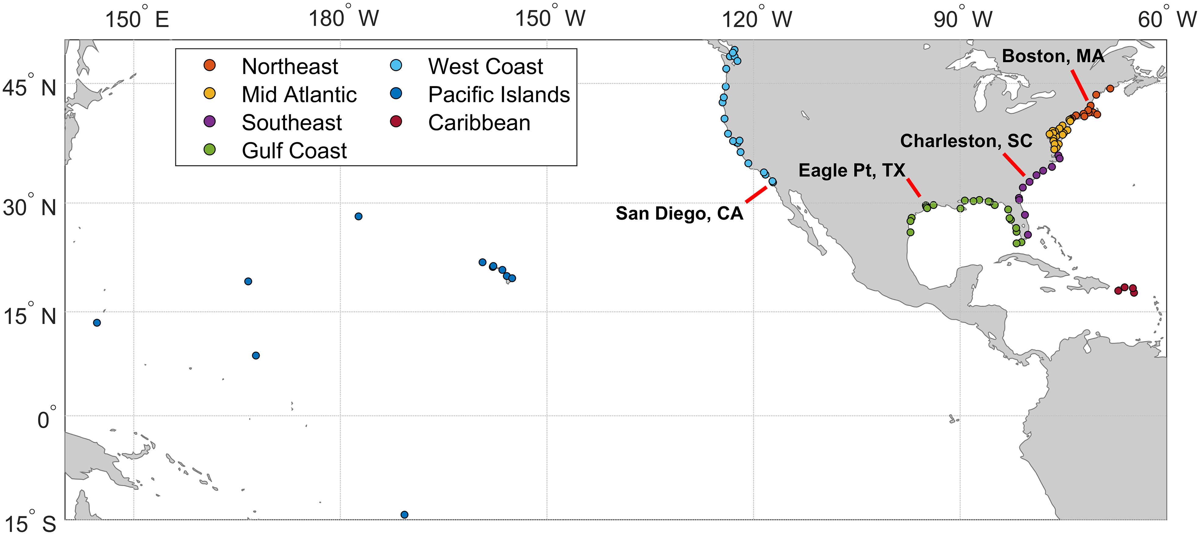
Figure 1 Map showing the 98 NOAA tide gauge locations used in the study color-coded by region used in the analysis (see legend). The location of four tide gauges used in detailed examples are indicated with labels and red lines.

Hourly tide predictions from 1997 – 2019 were calculated from NOAA stored and manually quality-assured tidal constituents (as described in Parker, 2007). Up to 37 standard tidal constituents are utilized, depending on which are statistically significant at each location. The tide predictions include both the SSA (solar semi-annual) and SA (solar annual) constituents, which typically resolve most of the seasonality at each gauge, however the long-term trend from sea level rise is not included. The NOAA tidal constituents are typically based on 5 years of observations with nodal factors applied utilizing an astronomical formula as described in Parker (2007), and were used in this study to maintain consistency with NOAA operational products.

NOAA tide predictions are standardized by referencing them to MHHW of the current tidal datum epoch (e.g. 1983 – 2001), regardless of what observational time period the constituents are calculated from. Thus, any relative sea level rise occurring since the center point of that epoch (usually 1992.5; Table S1) will not be accounted for in the tide predictions. To account for the long-term trend in relative sea level at each station, the linear trend in mean sea level (MSL) observed over the most recent 40 year period (1980-2019) was calculated (as in Zervas, 2009) and applied hourly to the tide predictions with an MSL of 0 at 1992.5, or the center point of the epoch. This method applies linear regression to the monthly mean MSL values with the seasonal MSL cycle removes to calculate the linear trend and corresponding 95% confidence limits.

A high tide flooding (HTF) occurrence equates to when the hourly observed water level exceeds the HTF threshold (Table S1), as described in Sweet et al. (2018). These thresholds were derived from National Weather Service minor flood thresholds, which were established at many NOAA tide gauges from years of flood-impact-monitoring. A linear fit between the empirical flood thresholds and tidal range at each NOAA tide gauge enabled calculating minor or HTF thresholds for all 98 gauges used in this study. The flooding thresholds typically range from 0.5 to 0.7 m above MHHW, except for in the tropical Pacific Islands including Hawaii where the thresholds are closer to 0.3 m above MHHW. Feedback from users and practitioners in the Pacific Islands have suggested that the nationally derived HTF thresholds are too high for Pacific Islands gauges. Observations support this assessment as the Sweet et al. (2018) thresholds have been exceeded rarely, if ever, for most Pacific Islands, despite numerous local reports of minor flooding. The thresholds for the 11 Pacific Island tide gauges are adjusted here by applying a regional fit derived from six of 11 gauges with existing local minor flood thresholds set by the National Weather Service (following the national method of Sweet et al., 2018). This results in regional thresholds about 20 cm lower than the national fit, and more closely aligned with what the National Weather Service has empirically established for the six gauges in this region.

Daily likelihood calculation

A prediction of the future daily HTF likelihood is based on the probability of exceedance occurring on a given day. The components of the hourly observed water level can be defined as:

where η_pred is the tide prediction, Δ_msl is the observed linear-trend change in MSL relative to the center of the last tidal epoch, and η_res is the non-tidal residual of observations with the linear-MSL trend excluded. A high tide flood day occurs when

where η_thresh is the HTF threshold for a particular tide gauge location (see Figure 2A for an example of the hourly observed water level, tide prediction, and flood threshold). Since η_pred and Δ_msl are a known or expected baseline water level, we can consider the freeboard, or the remaining water level until HTF occurs as:

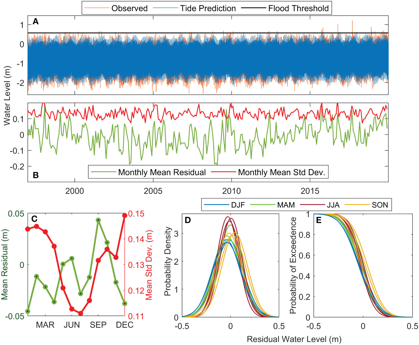
Figure 2 An example of the data preparation steps for Charleston, SC. The hourly observed water level (orange), SLR adjusted tide predictions (blue) and minor flood threshold (black line) relative to MHHW are shown (A). Plot (B) shows the monthly non-tidal residual µ (mean of hourly residuals; green) and σ (standard deviation of hourly residuals; red). Plot (C) shows the monthly average or climatological µ_clim (green) and σ_clim (red), and plots (D, E) show the probability density functions and cumulative distribution functions given those µ and σ for each month colored by season.

To determine the daily likelihood of a tide gauge exceeding η_thresh, we must calculate the probability of η_res >= Δ_free for some time t. To do this, we first calculated the hourly values of η_res for each gauge from 1997-2019. These data are then binned by calendar month and by decile of tide range for each gauge. Binning by month was done to account for observed seasonality in the residual. Binning by decile of tide range accounts for the observed dependence of the residual on tidal elevation, which is especially the case for many of the locations with larger tidal ranges (see Figure S1). This binning enables the determination of a climatological distribution of hourly η_res, with a climatological mean (µ_clim) and standard deviation (σ_clim) empirically calculated (see Figure 2B for an example).

The dependence of the residual on tidal elevation (i.e. for a specific water depth) is assumed to be independent of the time of year. If we calculate how µ_clim and σ_clim for a particular tidal elevation decile differ from the µ_clim and σ_clim for the entire data set, we can assume this broader relationship holds regardless of month. This enables the calculation of a tidal elevation adjustment factor for both µ_clim and σ_clim for a particular tidal elevation decile for each gauge:

where n is the length of the entire 23-year time series and n(i) represents the length of each tide elevation decile (i). The calculation of σ_adj follows the same convention but with standard deviation. Using this adjustment factor simplifies the calculation of µ_clim and σ_clim for a particular month and tidal decile, since it can be applied after the monthly calculations are made. As such, µ_clim and σ_clim are calculated for all 23 years of each calendar month (mo) and tidal elevation decile (i) as:

where $\overline{{\eta }_{res}}$ is the mean hourly residual of a given month and n(mo) represents the 23 calendar month values for each month for the entire 23-year analysis period (e.g., the mean residual from all 23 Januaries are averaged together; see Figure 2C). The calculation of σ_clim follows the same convention.

These calculations are made with the assumption that the residual distribution is normal. Although the extremes of the η_res distribution are not well fit by a normal distribution (Wahl et al., 2017), in this instance we are interested in the bulk of the distribution (i.e. 5% to 95% occurrence) where normality is a reasonable assumption (Ghanbari et al., 2019). A visual assessment indicates that a normal distribution function provides a reasonable estimation of the observed distribution (Figure S2).

From the climatological µ_clim and σ_clim a probability density function (PDF) f is calculated (as in Sweet and Park, 2014) for each calendar month (see Figure 2D) and each tide decile such that:

Then, the corresponding cumulative distribution function (CDF; see Figure 2E) for a normal distribution can be defined as:

where erf is the error function. The probability of exceedance P_hourly for a specific hourly freeboard water level Δ_free can then be calculated as:

Applying this function throughout the entire time series results in hourly exceedance probabilities from 1997-2019 (see Figure 2 for an example of the steps leading to this calculation). From a practical standpoint, we are most interested in the probability of flooding for a particular day. Thus, we calculate the cumulative probability of flooding for each 24-hour period to realize a daily prediction. The calculation of the daily cumulative probability is complicated by the temporal dependence of the hourly non-tidal residuals. To account for this dependence, we first calculate the autocorrelation, r, of the hourly η_res values, and the maximum probability for each day (P_max). The autocorrelation coefficient is then utilized to assess the dependence of each of the 23 remaining hourly values some time t away from the maximum probability for a given day. The cumulative daily probability P_daily is then calculated as:

Further, we assess persistence of the monthly MSL anomaly by performing an autocorrelation of monthly µ and σ anomaly (where the anomaly with the seasonal cycle removed is calculated by subtracting monthly µ_clim or σ_clim from the detrended monthly µ_obs and σ_obs) for the entire 23-year period at each of the 98 tide gauges. Persistent positive MSL anomalies have led to elevated periods of HTF in the past on both the U.S. East (Goddard et al., 2015) and West Coasts (Goodman et al., 2018), and strong persistence of the MSL anomaly has been shown for up to several seasons, especially in the tropical Pacific (Widlansky et al., 2017; Long et al., 2021). The assessment of persistence helps to determine if the MSL anomaly may be incorporated as an additional predictor in the model, and at what temporal lead time it might be reasonable to include persistence in a prediction. We perform such an assessment by comparing the skill performance for the persistence model to the baseline climatological model.

Skill assessment

Retrospective skill of HTF likelihoods at predicting when the HTF threshold, η_thresh, is exceeded is assessed by comparing the daily HTF likelihood to occurrences of daily maximum observed water level exceeding the threshold for each station from 1997 – 2019. The Brier Score (BS) is commonly used to assess skill of a probabilistic forecast (Wilks, 2019, Wilks, 2010) and is calculated as:

Where n is the time series length, t is the timestep, P is the HTF likelihood, and o is the observed flood occurrence (i.e., if η_thresh was not exceeded, then o = 0; and, if η_thresh was exceeded, then o = 1). BS is effectively the binary equivalent of mean squared error. BS is equal to zero if the HTF likelihood perfectly predicts flood occurrence and BS is equal to 1 if it is completely incorrect. We also compute the Brier Skill Score (BSS) as:

which relates the skill of the predicted HTF likelihood (BS) to the skill of the mean climatology reference prediction (BS_clim, which is a constant value calculated as the observed daily average HTF likelihood from 1997-2019). The BSS is used to determine how much of an improvement the HTF prediction is compared to the climatological mean. Standard error confidence intervals are calculated for the BSS as in Bradley et al. (2008). This method utilizes an analytical expression for BSS confidence intervals derived from sampling theory. Here we use the BSS standard error to provide a baseline level to determine if HTF predictions at a particular tide gauge location are skillful. HTF predictions made at a specific tide gauge location are deemed skillful when the BSS is greater than the BSS standard error.

A primary use case for these predictions is to warn of days where HTF is most likely to occur. As such, we designated a 5% threshold (i.e. P_t >= 0.05) as a potential HTF warning threshold. We then assess the recall (i.e., the fraction of observed HTF that were correctly predicted) and false-alarm-rate (FAR; i.e., the fraction of days without HTF that were incorrectly predicted to occur) for each tide gauge for the scenario of using the 5% threshold to predict HTF occurrence. The 5% threshold is also statistically relevant, as we cannot reasonably differentiate between the probabilities of extremes (i.e. events likely to occur less than 5% of the time), using a normal distribution of non-tidal residuals. Furthermore, accurately quantifying the likelihood of such extreme events is not the goal of our prediction method.

Assessing future potential flooding and skill

It is desirable to assess how model skill might change with future sea-level rise (SLR) given the acceleration of HTF occurrence even under relatively small rates of SLR. To accomplish this, we utilized the most recent 19 years of the data record (2001–2019) to provide representative observations for a complete tidal epoch, and then linearly detrended to remove the long-term sea level trend of the 19-year period. The mean of this 19-year observational period is then adjusted by the 40-year SLR trend at each station to simulate the sea level equivalent to both 2000 and 2020, and adjusted by the intermediate SLR scenario at each station to simulate the sea level likely by 2040 (Sweet et al., 2022). The intermediate scenario represents the downscaled, local relative SLR at specific tide gauge locations given a global MSL projection of 1 m of rise relative to a 2005 baseline. This scenario was chosen to represent a SLR amount that is likely for most U.S. coastal gauge locations based off of the regional tracking presented in Sweet et al. (2022).

Model predictions are made for each decade using the baseline climatological HTF model applied to the SLR adjusted 19-year observational period. A characteristic BSS is then calculated for each decade to assess how model skill will change with increasing SL.

Results

Climatological model

Retrospective predictive skill was assessed for the 92 tide gauges that observed at least 10 HTF days from 1997–2020 (Figure 3). The four stations in the Caribbean and two in the Florida Keys were excluded from model skill assessment because each station exceeded the HTF threshold three days or less. It is worth noting that this does not necessarily indicate that these locations do not experience more frequent flooding, rather, it is possible that flooding may occur when water level observed by the tide gauge does not exceed the HTF threshold. In these cases, flooding in regions near the tide gauge may be due to contributing factors such as waves and rainfall, and thus not well captured by observed mean water level.

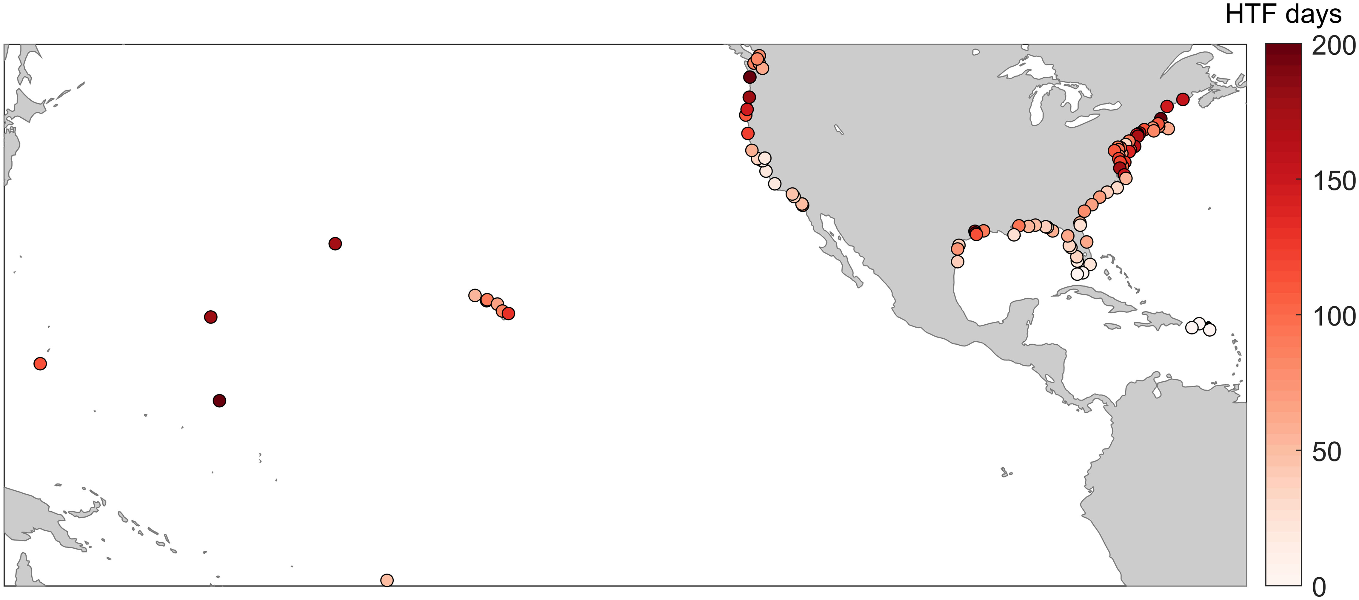
Figure 3 The total number of HTF days from 1997-2019 at each of the 98 NOAA tide gauges. Note that the days at some stations exceed 200.

The BSS serves as the primary metric to establish if the model predictions of HTF have skill when assessing observed flood days at each tide gauge. For 61 of the 92 gauges with at least 10 HTF days, the model demonstrated at least some skill (BSS > BSS Standard Error) when predicting observed HTF days, with the model demonstrating negative or negligible skill at the remaining 31 gauges (Figure 4A). In this case skillful values of BSS typically range between 0.01 – 0.5 and BSS Standard Errors typically range between 0.002 – 0.05. The model performed best along much of the West Coast, the Northeast Coast, and at several locations within the Southeast Coast as well as the Pacific Islands. The model generally performed poorly along the Gulf Coast, however skill minimally exceeded statistical significance at six of seven stations along the Texas Coast. Similarly, the model performance was poor and, in some cases, not skillful at a number of locations along the Mid-Atlantic Coast. In particular, the model was minimally skillful at only five of the 11 gauges in Chesapeake Bay and its tributaries (e.g., Washington, DC; Wachapreague, VA; and, Sewells Point, VA).

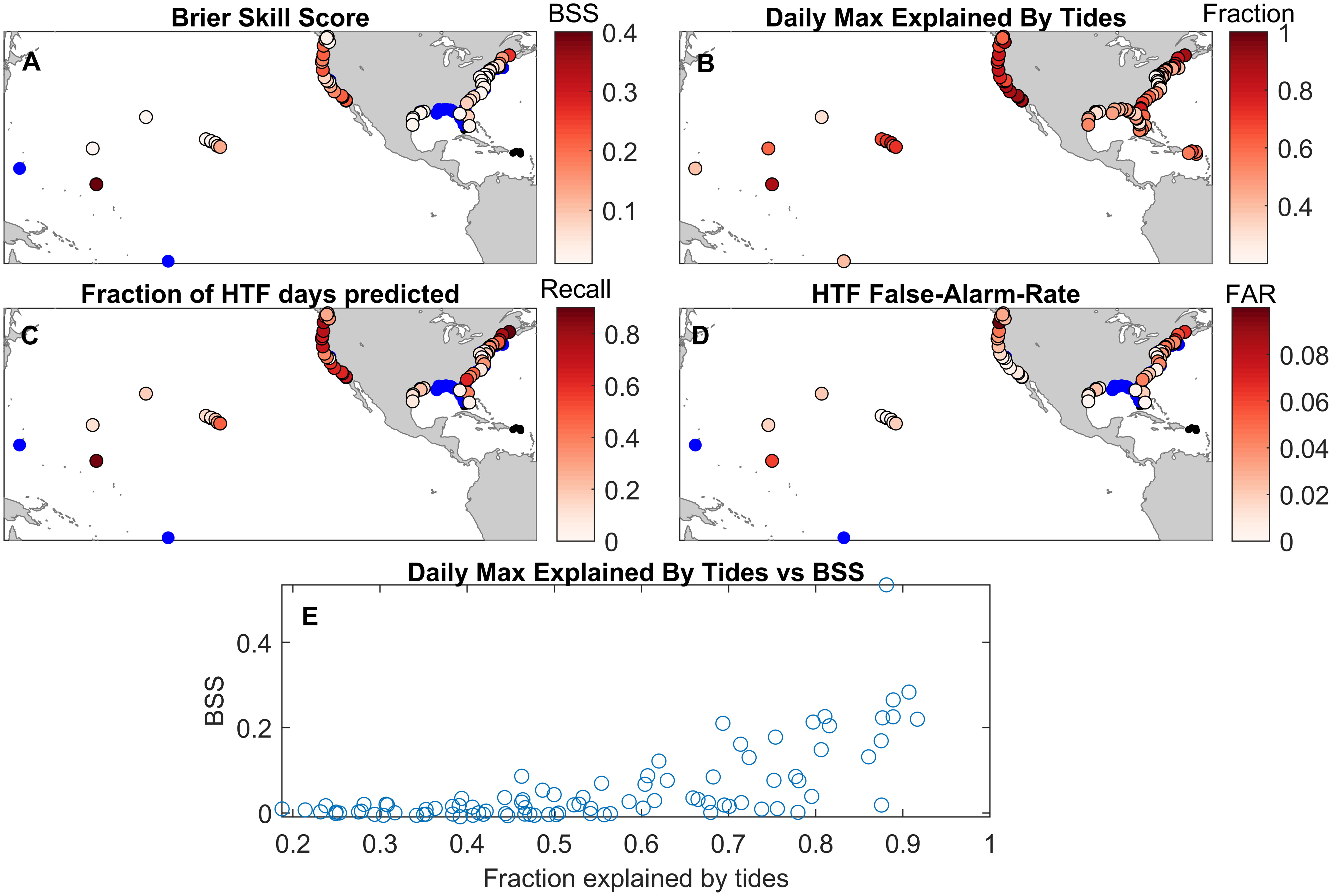
Figure 4 The Brier Skill Score (BSS) for each tide gauge (A). The fraction of the daily maximum observed water level variance explained by tides (B). The fraction of HTF days predicted when using a 5% warning threshold (C) and the false-alarm-rate when using that same 5% threshold (D). A scatter showing the relationship between BSS and the fraction of the daily max water level explained by tides is shown (E). In the maps, blue dots indicate insignificant skill (BSS< BSS Conf.), while small black dots (Caribbean and Florida Keys) indicate less than 10 HTF days occurred over the 1997 – 2019 period.

Poor model performance seems to be most prevalent in locations such as the Gulf of Mexico and Chesapeake Bay, which have relatively small tidal contributions to the daily maximum water level (Figure 4B, E). Although these locations have frequent floods, the high water-levels are often weather dominated and thus difficult to accurately predict with this model. Conversely, the locations with the greatest BSS are those where the tide accounts for a majority of the daily maximum water level variance. The skill dependence on tidal amplitude is expected, as the inherent skill in tide predictions is one of the primary reasons that this approach is viable. The 31 gauges with no retrospective skill as established by the BSS were not included in additional skill assessment metrics, since predictions would not be warranted at these locations.

The recall and false-alarm-rate applied to a 5% warning threshold of the model probabilities provides additional insight into the predictability of HTF events. The recall metric largely follows the same geographic patterns as the BSS, as a relatively high fraction of HTF days are correctly predicted at many locations in the West Coast, Northeast, parts of the Southeast, and several Pacific Islands (Figure 4C). For the 61 gauges demonstrating skill, on average 35% of all HTF days are accurately predicted using this model, with over half of HTF days accurately predicted at 18 gauges. Some of the best performing locations are discussed below.

In the Northeast, Bar Harbor, ME, Portland, ME and Boston, MA all experienced over 140 HTF days over the 23-year period, and the model impressively predicts more than 70% of HTF days accurately for Portland (71%), Boston (75%), and Bar Harbor (90%). Large numbers of HTF days also occurred along the northern West Coast, such as at Toke Point, WA and South Beach, OR (289 and 178 respectively) and there is similar good performance in flood prediction (78% and 74% accuracy rates, respectively). In southern California, San Diego and Santa Monica experienced a moderate number of flood days (74 and 45 respectively), with the model predictions accurately predicting 72% and 62% of HTF days for each location. Notable examples in the Southeast include Fort Pulaski, GA where the model predicted 62% of the 79 HTF days correctly and Charleston, SC which experienced 64 flood days and the model predicted 38% correctly. The model performed well at the Pacific Island stations at Kwajalein, Marshal Islands and Hilo, HI, where the model correctly predicted 87% of the more than 900 flood days at Kwajalein (note that the threshold may be leading to an overestimate of flood days at this location) and 47% of the 141 flood days at Hilo. Eagle Point, TX is the lone station in the Gulf with notable skill. Eagle Point experienced 273 flood days with many of these occurring over the past few years due to rapid regional land subsidence (Sweet et al., 2020). The model predicts 49% of these HTF days, despite the strong influence of weather along the Gulf of Mexico mentioned above. Importantly, the false-alarm-rate with this warning threshold was at 10% or less for nearly every tide gauge location that we considered.

We next examine more closely the example locations of Boston, MA, Charleston, SC, San Diego, CA and Eagle Point, TX. Reliability diagrams better express how the model performs relative to the observations over a range of probabilities (Figure 5). There is a clear imbalance of the distributions of probabilities. In each location, over 90% of predicted likelihoods are between 0 and 0.10. This is due in part to the fact that HTF days remain relatively infrequent, but also because in most locations, floods are unlikely unless the high tide is at least somewhat close to the flood threshold. Despite this imbalance, all four stations demonstrate fairly robust reliability across the entire range of predicted probabilities.

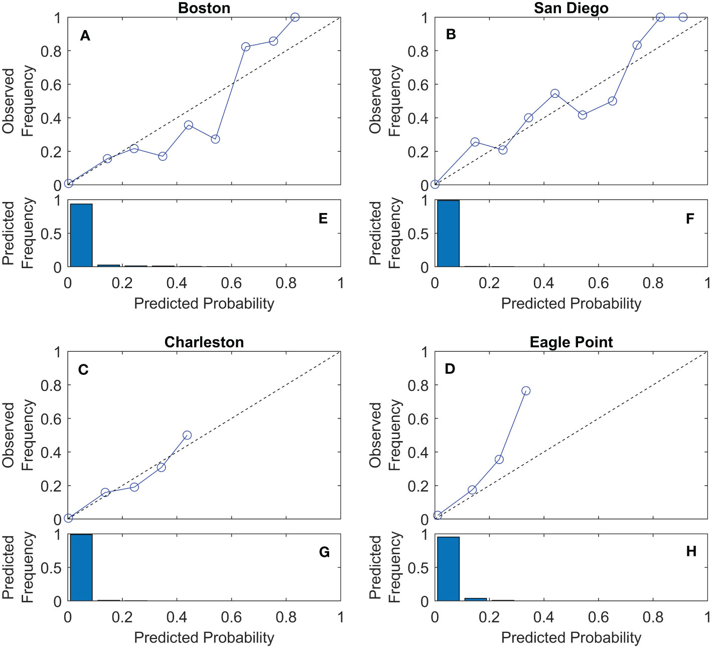
Figure 5 Reliability diagrams for Boston, MA, Charleston, SC, San Diego, CA, and Eagle Point, TX for retrospective daily HTF predictions from 1997 – 2019. Plots (A–D) show reliability relative to each predicted probability bin, where the x-axis location of each point is equal to the average of a particular probability bin. Plots (E–H) show the fraction of days predicted in each bin. Note that when no points are shown in a reliability diagram for a particular bin, this indicates 0 predicted probabilities in that bin, while all bins greater than 0.3 generally have too few observations to be visible in the bar plots.

The imbalanced distribution of predicted HTF likelihood is further evident in the model predictions for each of the four example stations during a sample year (e.g., 2017; Figure 6). The vast majority of days for all four gauges have a near-zero flood likelihood. However, there are several days with HTF likelihoods near 1 in these examples, especially for Boston and San Diego. Often, there are observed floods in such cases. This behavior demonstrates why a 5% HTF warning threshold is so robust—there are many days where flooding is improbable unless there is an extreme event—which by definition occurs infrequently. It is worth noting that model performance could be optimized by selecting a gauge-dependent warning threshold that may be less or greater than 5%, however the communication benefits and clarity of a uniform threshold likely outweighs those gains.

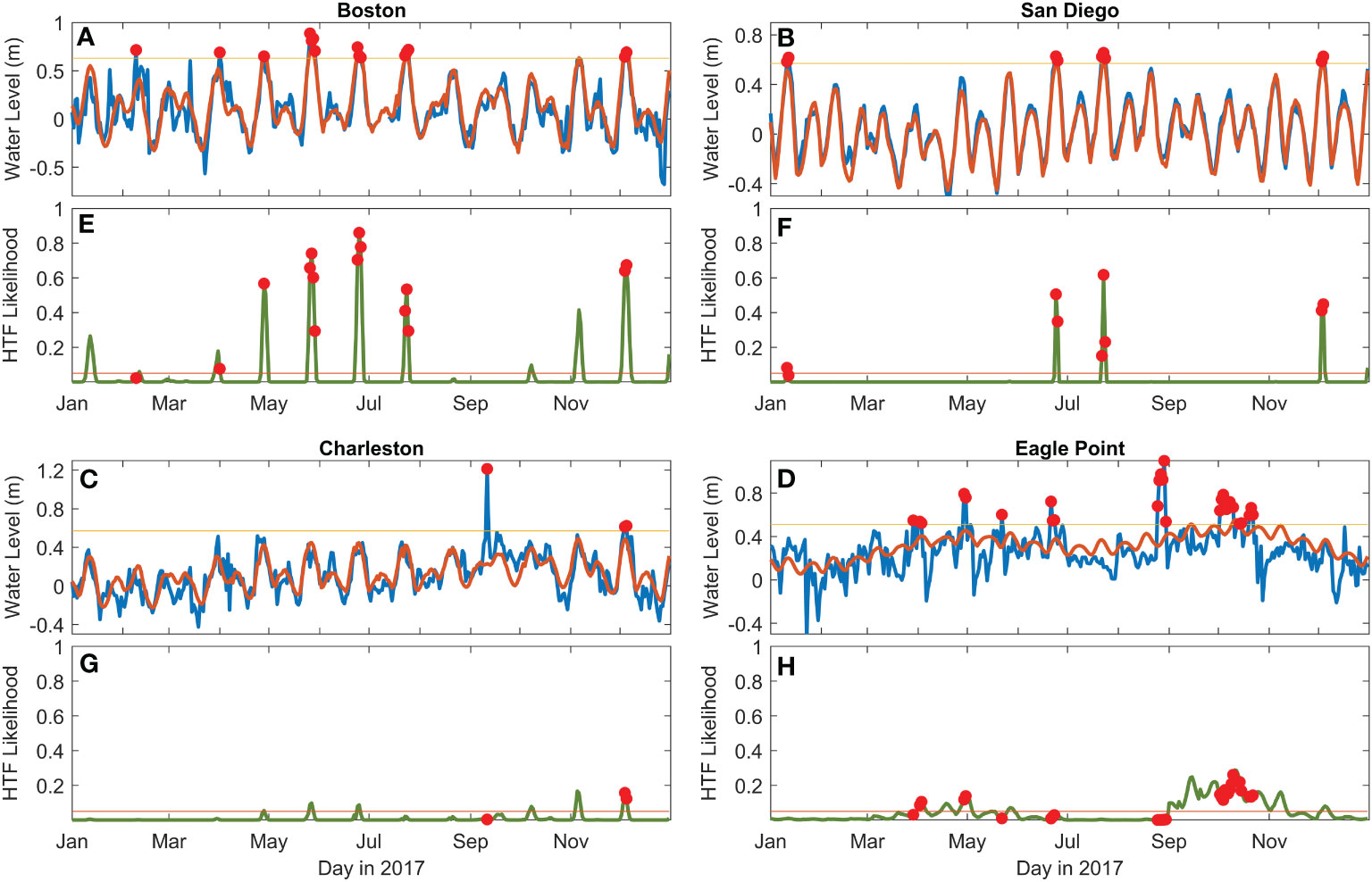
Figure 6 Time series examples of daily maximum observed (blue) and predicted (orange) water levels (A–D) and the daily HTF likelihood (green; E–H) for Boston, MA, Charleston, SC, San Diego, CA, and Eagle Point, TX for 2017. Red dots show days when HTF occurred and the horizontal yellow line shows the minor flood threshold (A–D) and 5% warning threshold (E–H).

The accuracy and potential value of using the climatological model to predict HTF events is clearly evident in the example year and locations. Using the 5% warning threshold during 2017, at Boston 14 of the 15 floods are predicted correctly, at San Diego 8 of 9 are predicted correctly, at Eagle Point 18 of 29 floods are predicted correctly, and at Charleston 2 of 3 are predicted correctly. The false-alarm rates were also relatively low (0.6% in San Diego, 4% in Charleston, 8% in Boston and 26% in Eagle Point).

Persistence model

Here, we investigate how the climatological model can be improved by including the damped persistence of the monthly MSL anomaly (µ_obs- µ_clim) as an additional predictor in our approach to predicting HTF events. First, we examine the autocorrelation of the monthly MSL anomaly (with the SL long-term trend removed) at each gauge. We consider the sea-level autocorrelations that exceed the positive 95% confidence limit of autocorrelations associated with a random process (i.e., white-noise) as being statistically significant (Figure 7A).

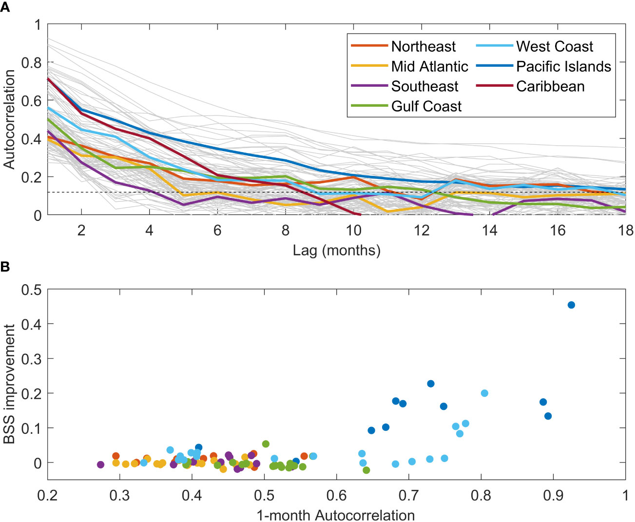
Figure 7 Autocorrelation of monthly MSL anomaly (A) for the 1997 – 2019 period for each of the 98 tide gauges (gray lines). The mean autocorrelation for each region (thick colored lines) and the positive 95% confidence limit of a white-noise autocorrelation (horizontal dashed line) are shown. Panel (B) shows the improvement in the BSS when using the 1-month damped persistence prediction compared to the climatological prediction (y-axis) as a function of the 1-month autocorrelation of monthly MSL anomaly (x-axis). Colors represent the same regions as in panel (A).

We find that all gauges have statistically significant autocorrelation at one-month lead, and most (91/98) have statistically significant autocorrelation at three-months lead. With the exception of the Pacific and Caribbean Islands, the autocorrelation falls off precipitously after this. Given this observation, and the fact that NOAA produces HTF guidance on seasonal time scales (i.e. three-months lead), including damped persistence at one- and three-month lead predictions were assessed for skill compared to the climatological-based model. Damped persistence was selected over simple persistence to account for the relatively rapid reduction in correlation between leads of 1 and 3 months at many stations and helps to reduce error at longer lead times. In our case, damped persistence is calculated simply as:

Where Δt is the lead time for the prediction (in this case 1 or 3 months), r is the normalized autocorrelation and f’(t) is the monthly MSL anomaly.

Autocorrelation at 1 month was greatest for the Pacific and Caribbean Islands and along parts of the West Coast (Figure 7, Figure 8A). The locations with greater autocorrelation generally see the largest improvements in skill, with fairly substantial BSS improvements at most Pacific Island gauges and also in the southern West Coast (Figures 7B, 8C, D). Eight of the 11 Pacific Island stations had a 1-month BSS increase of greater than 0.1 when compared to the climatological model. This improvement is also reflected in the recall (Figurse 8E, F), as these same stations had at least a 30% improvement in predicting positive HTF days. The Pago Pago, AS gauge saw the greatest improvement across the entire network, with BSS increasing by 0.45 and recall improving by a dramatic 84%. The 1-month persistence prediction in San Diego, CA improved upon the climatological model by a BSS of 0.20 (largest improvement in the continental U.S.) and by a recall of 15%, while gauges at La Jolla, Los Angeles and Santa Monica, CA all saw 1-month BSS improvements of at least 0.08 and recall improvements of at least 14%. Outside of these regions, improvements in BSS and recall at 1-month lead are much subtler or even negligible. Only 29 of the 98 gauges saw a statistically significant improvement in BSS at the 1-month lead, and only 16 of the 84 gauges not on the Pacific or Caribbean Islands. For these 16 gauges on the Continental U.S. Coast, except for those in Southern California where the autocorrelations are relatively high, recall improvements were generally only a few percent.

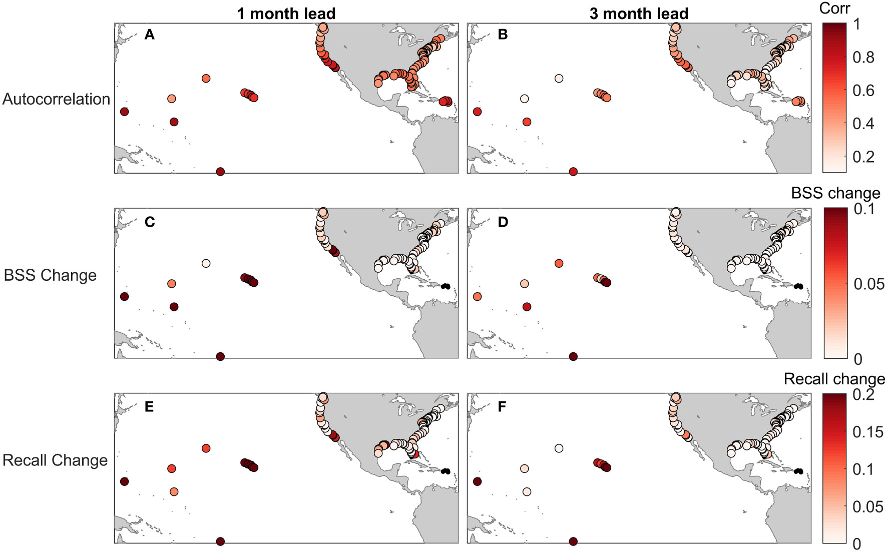
Figure 8 Shown are the autocorrelation of monthly MSL anomalies at both 1 and 3 months of lead (A, B) and the change in BSS (C, D) or recall (E, F) when using the monthly MSL anomaly for the prediction of HTF days at either one- or three-months lead. Small black dots in the BSS and Recall plots (Caribbean and Florida Keys) indicate less than 10 HTF days occurred over the 1997 – 2019 period.

The autocorrelation at lead 3 months was obviously less (Figure 8B), but similarly greatest in the Pacific and Caribbean Islands and Southern California, with generally minimal correlation elsewhere. Improvements in BSS at 3-month lead were quite a bit lower in most cases (Figure 8D), but still significant, with improvements in the Pacific Islands ranging from 0.01 to 0.15 BSS (recall improvements of 0 to 57%). On the West Coast, improvements were mostly negligible (i.e., not statistically significant) except for San Diego, where the BSS improved by 0.09 and the recall by 8%. Overall, and besides the tide gauges in the Pacific and Caribbean Islands, including the sea level autocorrelation information at lead 3 months was associated with mostly negligible skill improvements (only six locations in the Continental U.S. had statistically significant increases in BSS).

Model skill improvements due to relative sea level rise

The implications of sea level rise on model performance can be assessed by applying the climatological model to a detrended 19-year (2001 – 2019) representative time series with adjusted mean sea level (MSL). Here, MSL is adjusted by the 40-year station specific SL trend to simulate sea levels in 2000 and 2020 and adjusted by the decadal Intermediate SLR scenarios to simulate sea levels likely in 2040 (Sweet et al., 2022). For most gauges, BSS increases with increasing SLR from 2000 to 2040 (Figure 9), with the exception of the Caribbean stations, which do not have a sufficient number of floods to assess skill, even with SLR. For relative sea levels typical in 2000, only 42/92 gauges (outside of the Caribbean and Florida Keys) have skillful HTF predictions. For sea levels typical in 2020, 68/92 gauges demonstrate skill and by 2040, projections suggest that skillful HTF predictions can be made at 93/94 gauges (which now includes the two Florida Key gauges).

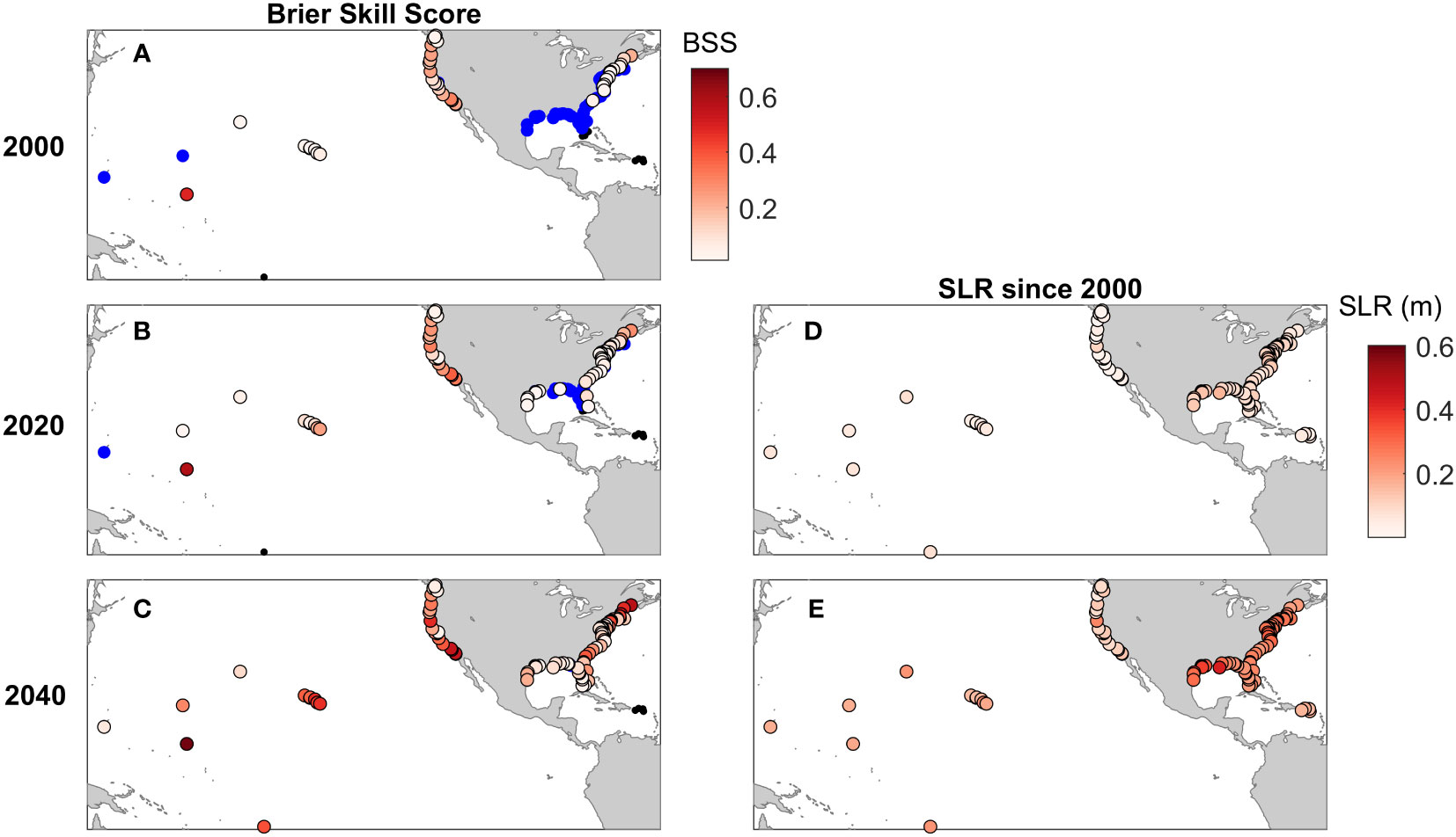
Figure 9 Brier Skill Scores for HTF predictions made assuming mean sea level (MSL) is equivalent to the detrended mean at about 2000 (A) and 2020 (B) and for the intermediate SLR projection for 2040 (C). Blue dots indicate insignificant skill (BSS< BSS Conf.), while small black dots (e.g. Caribbean and Florida Keys) indicate less than 10 HTF days occurred over the MSL adjusted 19-year period. The estimated SLR since 2000 is shown for 2020 (D) and the intermediate SLR projection for 2040 is shown (E).

This improvement occurs due to SLR reducing the amount of non-tidal residual necessary to exceed the HTF threshold on any given day. The increase in MSL results in a substantially greater number of days with at least some chance of flooding, as the median number of days per year exceeding the 5% warning threshold across all gauges goes from 0 in 2000, to 7.5 in 2020 to 78.5 in 2040. Since the increase in likely flood days by 2040 is so large, using a warning threshold larger than 5% in the future may be beneficial to reduce false alarms and excessive warning of possible flood events. Further, the number of days per year when flooding will occur without any non-tidal residual contribution goes from a median of 0 in 2000 and 2020 (i.e. most stations have no flooding due to tides alone) to a median of 7 in 2040. These results indicate that model skill will increase as flooding becomes increasingly less dependent on weather and climate driven variability; and, instead, tidal variability becomes an even more important predictor of flooding.

The impact of these changes in flood likelihood with increasing SLR on a warning product is evident in Figure 10. Using the same four example stations as previously considered, elevated flooding likelihood goes from a very infrequent occurrence in 2000, to high likelihood floods several days per month in 2040. In the case of Eagle Point, flooding will be likely in 2040 nearly every day according to the HTF threshold that we used.

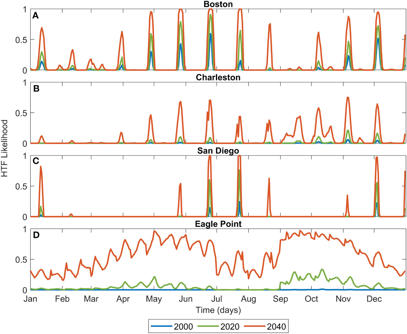
Figure 10 Examples of HTF prediction at Boston, MA (A), Charleston, SC (B), San Diego, CA (C) and Eagle Point, TX (D) for one year assuming MSL at levels observed in 2000 (blue), 2020 (green) and projected with the Intermediate Scenario for 2040 (orange).

Discussion

We demonstrated that a new HTF predictive model has retrospective skill at many U.S. coastal locations. The innovation is combining astronomical tide predictions, either climatological non-tidal residuals or persisting SL anomalies, and long-term MSL changes to produce the HTF predictions. The climatology-based model demonstrates at least some skill for 61 of the 92 tide gauges where at least 10 HTF days were observed from 1997 – 2019. Including observed characteristics about the persistence of SL anomalies further improves the skill at many locations for producing near-term predictions (i.e., leads of 1 – 3 months). Ongoing SLR will increasingly dominate the determination of HTF occurrence, and hence continue to increase the prediction skill (skillful at 93/94 stations with regular flooding by 2040), if the assumption is made that flood thresholds are not increased due to successful mitigation measures.

At many locations along the U.S. West Coast (e.g., San Diego) and Northeast Coast (e.g., Boston), the HTF prediction model was successful even when relying on the climatological non-tidal residual. Prediction skill in these regions is in part due to the importance of high tides to cause flooding, versus weather forcing and other drivers of SL anomalies (Figure 4 see also Sweet et al., 2018). At many locations along the West and Northeast Coasts, tidal predictions already resolve much of the observed water level (much of the variability is related to the sea level annual cycle; e.g., Widlansky et al., 2020). Hence, it follows that an HTF prediction informed primarily by tide predictions that includes the annual cycle will perform well for these locations.

Conversely, tidal contributions to HTF are relatively small for some other locations such as along the Gulf of Mexico and in the Mid-Atlantic (e.g., Chesapeake Bay). In such locations, water level variability is much more dependent on weather events and climate variability (Figure 4; see also Sweet et al., 2018). As such, the HTF prediction model lacks skill at many locations along the Gulf of Mexico and in the Mid-Atlantic. However, with continuing SLR, high tides alone will more frequently approach or exceed the current HTF threshold. As weather-forced water level variability becomes relatively less important to causing HTF exceedance, this method will begin to be skillful across most, if not all of the U.S. coastline (Figure 9).

Considering locations experiencing land subsidence and associated relative SLR provides a contemporary example for how the HTF prediction model may be useful, even for regions that are less tidally driven, such as along the Gulf of Mexico and Chesapeake Bay. During 2018 and 2019, the tide gauge at Eagle Point, TX observed the greatest number of HTF days (85) at any location on the Gulf Coast. The recent HTF events are primarily due to localized subsidence in the vicinity of the gauge leading to rapid relative SLR of about 1.4 cm/year over the last 26 years (Sweet et al., 2020). In fact, there is already a nearly constant threat of daily flooding in the months of September and October at Eagle Point, TX (Figure 6). The rapid rate of SLR there is somewhat of a preview for how flooding at other locations may respond to SLR later this century.

Including MSL persistence significantly improves skill for 1-month lead at 29 tide gauge locations, including in most of the Pacific Island gauges. The locations with the greatest improvement in skill are, not surprisingly, those with high autocorrelation in the monthly MSL anomaly (Figure 7). An additional benefit of applying the persistence forecast is that it enables accounting for errors in the long-term MSL trend or contemporary deviations in MSL away from the historic fit. An example of a changing sea level trend is occurring at the Pago Pago, AS, where acceleration in rising relative MSL due to land subsidence occurred following a major earthquake in 2009 (Han et al., 2019). Including persistence helps to better account for this recent change in the MSL trend and resulted in a 0.45 improvement in BSS compared to the climatological model, which was the largest improvement across all 98 gauges. It is possible that errors in the MSL trend or deviations from the long-term linear MSL trend could be further mitigated by utilizing shorter-term MSL fits, or also applying confidence bounds to MSL values, which are approaches that should be explored in future work.

The HTF prediction model capabilities will improve the approaches NOAA utilizes to provide guidance regarding potential future HTF days. For the annual outlooks NOAA already regularly produces, the climatological modeling approach can be used to identify specific dates where HTF is most likely, which is information not presently available from the existing trend-based method. For the NOAA seasonal High Tide Bulletins (https://oceanservice.noaa.gov/news/high-tide-bulletin/), this new HTF prediction model will enable quantifying daily HTF likelihood for specific tide gauge locations. This information would substantially improve existing capabilities, which only provide qualitative guidance of likely flooding days for broad regions of the coast (e.g. suggesting days HTF is most likely for the Northeast U.S. Coast). The persistence model can also be applied with a one- to three-month lead time to provide more accurate seasonal predictions for many locations. This information could be conveyed to the public using an enhanced tidal calendar (e.g., as pictured in Figure 11). Such an HTF calendar outlook, would better convey when and where coastlines are likely to be impacted by the combined occurrence of high tides, above-normal sea levels, and long-term SLR. A similar HTF calendar approach has been developed for many tropical Pacific Islands (Widlansky et al., 2017), but does not yet exist elsewhere.

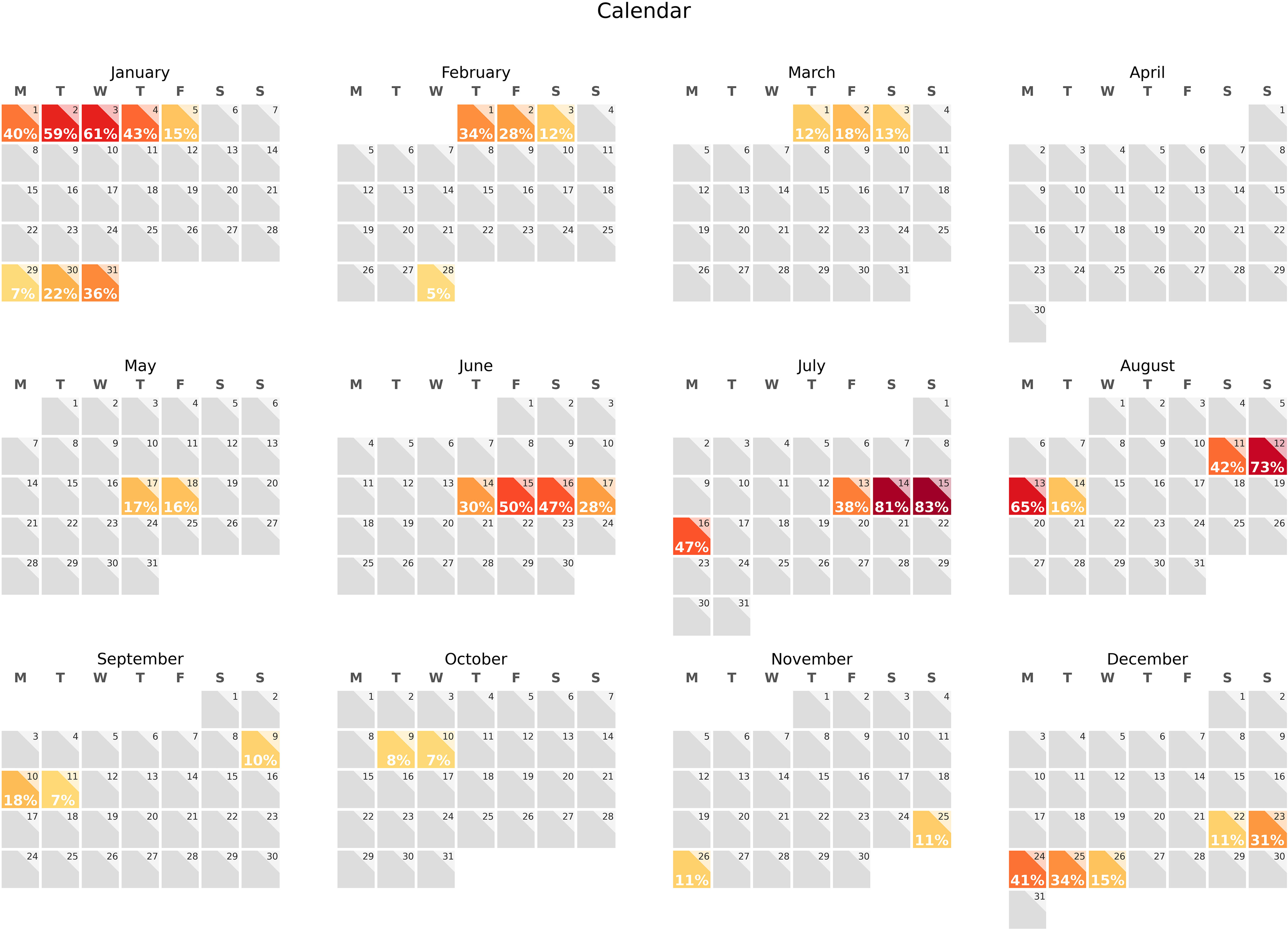
Figure 11 An example visualization product of the HTF likelihood for Charleston, SC during 2018. Color shading indicates days that exceed the 5% warning threshold (yellow, near 5%; red, near 100%) with the HTF likelihood listed.

Part of the motivation for this work is to provide a baseline level of HTF prediction skill for future numerical, statistical or machine learning (ML) model development. To this end, any future MSL anomaly prediction efforts must be able to improve upon the persistence predictions utilized here. Modeled MSL anomaly has been demonstrated to improve upon persistence for most of the tropical Pacific Islands, especially at leads of one-to-two seasons (Miles et al., 2013; McIntosh et al., 2015; Widlansky et al., 2017; Jacox et al., 2020). Utilizing multi-model ensembles has been demonstrated to result in skillful MSL anomaly predictions at many global locations (Long et al., 2021), including in the Pacific Islands, throughout the Caribbean Sea, as well as parts of the U.S. West Coast. Initial research utilizing an ML approach to predict MSL anomalies along the continental U.S. demonstrated some retrospective skill, especially along the West Coast (Sheridan et al., 2019). The capability for skillful anomaly predictions along the U.S. East and Gulf Coasts is so far less evident, however recent model advancements show that some skill is possible for lead times up to a few months (Shin and Newman, 2021; Frederikse et al., 2022). Further examination of these approaches, especially as applied to the prediction of HTF days, is essential to assess the potential value to NOAA HTF decision-support products. The method presented here provides the product infrastructure necessary to make these determinations about future forecasting advancements. We anticipate that modeled-based MSL anomalies will be “plugged-in” to this method and then compared to the skill of the climatological and persistence approaches, to determine the best-available sea level outlook at a particular location.

It is important to note that the assessment of HTF flooding occurrence as presented here is dependent on relating tide gauge point observations to empirically derived flood thresholds (Sweet et al., 2018). Spatial variations in coastal water level variability is in some places significant, especially in enclosed bays and estuaries (Aretxabaleta et al., 2019), and thus flooding even a short distance away from the tide gauge may not be accurately reflected by these observations. The position of the tide gauge also may not well capture freshwater contributions (i.e., associated with precipitation, runoff, and flow from rivers or canals). Hydrologic forcing can lead to flooding on its own or contribute to existing tidal flooding (Wdowinski et al., 2016; Sukop et al., 2018). In addition, existing flood thresholds may not best reflect similar levels of impact everywhere. For instance, a threshold exceedance in Maine may result in substantially different impacts than one in South Florida due to differences in coastal topography and exposed infrastructure. Lastly, this assessment is based on hourly sub-sampled six-minute mean water level values, and thus will only account for time-averaged wave contributions to water level, and not higher frequency time-varying contributions. Wave contributions to flooding (e.g. wave runup) are known to be important, especially along the U.S. West Coast and Pacific Islands (Serafin et al., 2017; Barnard et al., 2019). These limitations can be overcome, although advancement will require additional observations and numerical modeling to better assess spatial variations in coastal flooding and resultant impacts.

Lastly, it is important to recognize the limitations with the approach utilized to assess the influence of SLR on the skill of this model. We chose a simple mean shift of existing observations to provide a first-order assessment of the contributions of SLR to model skill. This approach does not account for future flood mitigation efforts, which would hopefully raise the HTF thresholds. It also does not account for potential changes sea level variability due to future warming or atmospheric changes (Widlansky et al., 2020), nor future changes in the tides due to either SLR or alterations of the local bathymetry or topography (Devlin et al., 2017; Talke and Jay, 2020). These contributions, coupled with deviations of RSL rise from the Intermediate Scenario estimate utilized here, as well as intra-decadal astronomical tidal variability (Thompson et al., 2021), could alter the projected future HTF frequency and likelihood.

Conclusions

In this paper, we found that a simple model including tide predictions, relative SLR, and climatological monthly non-tidal residuals has retrospective skill in predicting HTF likelihood. We demonstrated skill of this approach at 61 out of 92 NOAA tide gauges where at least 10 HTF days occurred during 1997 – 2019. With the realization of RSL rise over the next several decades, the same approach is likely to be skillful at 93 out of 94 gauges with regular flooding assuming unchanging HTF thresholds in the future. Further, if the observed persistence of SL anomalies is included, model skill can be significantly improved at many locations, especially in the Pacific Islands and U.S. West Coast. These results demonstrate that this approach has value to provide many coastal communities with decision-support information right now.

This approach also has the flexibility to be enhanced as research improves our ability to predict coastal water level anomalies. For instance, the statistical model that we developed has the benefit of being agnostic to the method for estimating the MSL anomaly used to generate the HTF predictions. Thus, any modeling infrastructure developed to run this model operationally will be well positioned to include MSL anomaly output from future numerical, statistical, or ML models. Further, it would be simple to regionalize this approach and use variable input depending on location (e.g., the West Coast may use an MSL anomaly prediction from a numerical model, whereas the Gulf Coast may rely solely on persistence). This flexibility will ensure that efforts to operationalize the baseline HTF predictive approach will both provide immediate near-term benefits, while well positioning NOAA products like the High Tide Bulletin for future improvements to model skill from advancements in our ability to accurately model MSL anomalies along more of the U.S. Coast (e.g., Frederikse et al., 2022). Additionally, the use of model analyses or satellite observations could enable HTF predictions to be extended away from tide gauge locations and be provided continuously along coastlines, thus further enhancing the utility of predictions for coastal communities.

Data availability statement

Publicly available datasets were analyzed in this study. This data can be found here: https://tidesandcurrents.noaa.gov/web_services_info.html.

Author contributions

GD performed all analyses, plots and wrote most of the text of the manuscript. WS provided code, information regarding flood thresholds and sea level scenarios and assisted with analysis. MW and PT provided guidance on methods. JM provided support on Pacific Island flood thresholds. All authors contributed to the article and approved the submitted version.

Funding

MW was supported by the NOAA Climate Program Office’s Modeling, Analysis, Predictions, and Projections (MAPP) program through grants NA17OAR4310110 and NA22OAR4310138. PT was supported by the NOAA ResearchGlobal Ocean Monitoring and Observing Program via the University of Hawaii Sea Level Center (Grant No. NA16NMF4320058).

Acknowledgments

The authors would like to thank Peter Stone and Bob Heitsenrether for their review and suggested improvements to this manuscript. We would also like to thank Dr. Chris Zervas for his support in providing estimates of relative sea level rise at each NOAA tide gauge.

Conflict of interest

The authors declare that the research was conducted in the absence of any commercial or financial relationships that could be construed as a potential conflict of interest.

The reviewer SL declared a past collaboration with one of the authors PT to the handling Editor.

Publisher’s note

All claims expressed in this article are solely those of the authors and do not necessarily represent those of their affiliated organizations, or those of the publisher, the editors and the reviewers. Any product that may be evaluated in this article, or claim that may be made by its manufacturer, is not guaranteed or endorsed by the publisher.

Supplementary material

The Supplementary Material for this article can be found online at: https://www.frontiersin.org/articles/10.3389/fmars.2022.1073792/full#supplementary-material

References

American Meteorological Society (2022). Glossary of meteorology. Available at: http://glossary.ametsoc.org/wiki/High_tide_flooding.
Aretxabaleta A. L., Ganju N. K., Defne Z., Signell R. P. (2019). Spatial distribution of water level impacting back-barrier bays. Natural Hazards Earth System Sci. 19, 1823–1838. doi: 10.5194/nhess-19-1823-2019
Barnard P. L., Erikson L. H., Foxgrover A. C., Hart J. A. F., Limber P., O’neill A. C., et al. (2019). Dynamic flood modeling essential to assess the coastal impacts of climate change. Sci. Rep. 9, 1–13. Available at: https://doi.org/10.1038/s41598-019-40742-z
Bradley A. A., Schwartz S. S., Hashino T. (2008). Sampling uncertainty and confidence intervals for the brier score and brier skill score. Weather Forecasting 23, 992–1006. doi: 10.1175/2007WAF2007049.1
Buchanan M. K., Oppenheimer M., Kopp R. E. (2017). Amplification of flood frequencies with local sea level rise and emerging flood regimes. Environ. Res. Lett. 12, 064009. doi: 10.1088/1748-9326/aa6cb3
Burgos A. G., Hamlington B. D., Thompson P. R., Ray R. D. (2018). Future nuisance flooding in Norfolk, VA, from astronomical tides and annual to decadal internal climate variability. Geophysical Res. Lett. 45, 12,432–12,439. doi: 10.1029/2018GL079572
Dahl K. A., Fitzpatrick M. F., Spanger-Siegfried E. (2017). Sea Level rise drives increased tidal flooding frequency at tide gauges along the U.S. East and gulf coasts: Projections for 2030 and 2045. PloS One 12, e0170949. doi: 10.1371/journal.pone.0170949
Devlin A. T., Jay D. A., Zaron E. D., Talke S. A., Pan J., Lin H. (2017). Tidal variability related to Sea level variability in the pacific ocean. J. Geophysical Res.: Oceans 122, 8445–8463. doi: 10.1002/2017JC013165
Fraser R., Palmer M., Roberts C., Wilson C., Copsey D., Zanna L. (2019). Investigating the predictability of north Atlantic sea surface height. Climate Dynamics 53, 2175–2195. doi: 10.1007/s00382-019-04814-0
Frederikse T., Lee T., Wang O., Kirtman B., Becker E., Hamlington B., et al. (2022). A hybrid dynamical approach for seasonal prediction of Sea-level anomalies: A pilot study for Charleston, south Carolina. J. Geophysical Res.: Oceans 127, 1–17. Available at :https://doi.org/10.1029/2021JC018137
Ghanbari M., Arabi M., Obeysekera J., Sweet W. (2019). A coherent statistical model for coastal flood frequency analysis under nonstationary Sea level conditions. Earth's Future 7, 162–177. doi: 10.1029/2018EF001089
Gill S., Hovis G., Kriner K., Michalski M. (2014). “Implementation of procedures for computation of tidal datums in areas with anomalous trends in relative mean Sea level,” in NOAA Technical report (Silver Spring, MD: NOAA).
Gill S. K., Schultz J. R. (2000). “Tidal datums and their applications,” in NOAA Special publication (Silver Spring, MD: National Oceanic and Atmospheric Adminstration).
Goddard P. B., Yin J., Griffies S. M., Zhang S. (2015). An extreme event of sea-level rise along the northeast coast of north America in 2009–2010. Nat. Commun. 6, 6346. doi: 10.1038/ncomms7346
Goodman A. C., Thorne K. M., Buffington K. J., Freeman C. M., Janousek C. N. (2018). El Niño increases high-tide flooding in tidal wetlands along the U.S. pacific coast. J. Geophysical Res.: Biogeosci. 123, 3162–3177. Available at: https://doi.org/10.1029/2018JG004677
Han S. C., Sauber J., Pollitz F., Ray R. (2019). Sea Level rise in the Samoan islands escalated by viscoelastic relaxation after the 2009 Samoa-Tonga earthquake. J. Geophysical Res.: Solid Earth 124, 4142–4156. doi: 10.1029/2018JB017110
Hino M., Belanger S. T., Field C. B., Davies A. R., Mach K. J. (2019). High-tide flooding disrupts local economic activity. Sci. Adv. 5, eaau2736. doi: 10.1126/sciadv.aau2736
Hummel M. A., Berry M. S., Stacey M. T. (2018). Sea Level rise impacts on wastewater treatment systems along the U.S. coasts. Earth's Future 6, 622–633. doi: 10.1002/2017EF000805
Jacobs J. M., Cattaneo L. R., Sweet W., Mansfield T. (2018). Recent and future outlooks for nuisance flooding impacts on roadways on the U.S. East coast. Transportation Res. Record: J. Transportation Res. Board 2672, 1–10. doi: 10.1177/0361198118756366
Jacox M. G., Alexander M. A., Siedlecki S., Chen K., Kwon Y.-O., Brodie S., et al. (2020). Seasonal-to-interannual prediction of north American coastal marine ecosystems: Forecast methods, mechanisms of predictability, and priority developments. Prog. Oceanography 183, 102307. doi: 10.1016/j.pocean.2020.102307
Keenan J. M., Hill T., Gumber A. (2018). Climate gentrification: from theory to empiricism in Miami-Dade county, Florida. Environ. Res. Lett. 13, 1–11. doi: 10.1088/1748-9326/aabb32
Kopp R. E., Gilmore E. A., Little C. M., Lorenzo-Trueba J., Ramenzoni V. C., Sweet W. V. (2019). Usable science for managing the risks of Sea-level rise. Earth's Future 7, 1235–1269. doi: 10.1029/2018EF001145
Kopp R. E., Horton R. M., Little C. M., Mitrovica J. X., Oppenheimer M., Rasmussen D. J., et al. (2014). Probabilistic 21st and 22nd century sea-level projections at a global network of tide-gauge sites. Earth's Future 2, 383–406. doi: 10.1002/2014EF000239
Long X. Y., Widlansky M. J., Spillman C. M., Kumar A., Balmaseda M., Thompson P. R., et al. (2021). Seasonal forecasting skill of Sea-level anomalies in a multi-model prediction framework. J. Geophysical Res.-Oceans 126. doi: 10.1029/2020JC017060
McAlpine S. A., Porter J. R. (2018). Estimating recent local impacts of Sea-level rise on current real-estate losses: A housing market case study in Miami-Dade, Florida. Population Res. Policy Rev. 37, 871–895. doi: 10.1007/s11113-018-9473-5
McIntosh P. C., Church J. A., Miles E. R., Ridgway K., Spillman C. M. (2015). Seasonal coastal sea level prediction using a dynamical model. Geophysical Res. Lett. 42, 6747–6753. doi: 10.1002/2015GL065091
Miles E. R., Spillman C. M., Church J. A., Mcintosh P. C. (2014). Seasonal prediction of global sea level anomalies using an ocean–atmosphere dynamical model. Climate Dynamics 43, 2131–2145. doi: 10.1007/s00382-013-2039-7
Miles E. R., Spillman C. M., Mcintosh P. C., Church J. A., Charles A. N., De Wit R. (2013). “Seasonal Sea-level predictions for the Western pacific,” in Conference: 20th International Congress on Modelling and Simulation, Adelaide, Australia.
Moftakhari H. R., Aghakouchak A., Sanders B. F., Matthew R. A. (2017b). Cumulative hazard: The case of nuisance flooding. Earth's Future 5, 214–223. doi: 10.1002/2016EF000494
Moftakhari H., Aghakouchak A., Sanders B. F., Matthew R. A., Mazdiyasni O. (2017a). Translating uncertain Sea level projections into infrastructure impacts using a Bayesian framework. Geophysical Res. Lett. 44, 11,914–11,921. doi: 10.1002/2017GL076116
Obeysekera J., Irizarry M., Park J., Barnes J., Dessalegne T. (2011). Climate change and its implications for water resources management in south Florida. Stochastic Environ. Res. Risk Assess. 25, 495–516. doi: 10.1007/s00477-010-0418-8
Serafin K. A., Ruggiero P., Stockdon H. F. (2017). The relative contribution of waves, tides, and non-tidal residuals to extreme total water levels on US West coast sandy beaches. Geophysical Res. Lett. Vol 44, 1839–47. doi: 10.1002/2016GL071020
Sheridan S. C., Lee C. C., Adams R. E., Smith E. T., Pirhalla D. E., Ransibrahmanakul V. (2019). Temporal modeling of anomalous coastal Sea level values using synoptic climatological patterns. J. Geophysical Res.: Oceans 124, 6531–6544. doi: 10.1029/2019JC015421
Shin S. I., Newman M. (2021). Seasonal predictability of global and north American coastal Sea surface temperature and height anomalies. Geophysical Res. Lett. 48, , 1–10. doi: 10.1029/2020GL091886
Stephens S. A., Bell R. G., Ramsay D., Goodhue N. (2014). High-water alerts from coinciding high astronomical tide and high mean Sea level anomaly in the pacific islands region. J. Atmospheric Oceanic Technol. 31, 2829–2843. doi: 10.1175/JTECH-D-14-00027.1
Sukop M. C., Rogers M., Guannel G., Infanti J. M., Hagemann K. (2018). High temporal resolution modeling of the impact of rain, tides, and sea level rise on water table flooding in the arch creek basin, Miami-Dade county Florida USA. Sci. Total Environ. 616, 1668–1688. doi: 10.1016/j.scitotenv.2017.10.170
Sweet W., Dusek G., Carbin G., Marra J., Marcy D., Simon S. (2020). “2019 state of U.S. high tide flooding with a 2020 outlook,” in NOAA Technical report (Silver Spring, MD: NOAA).
Sweet W., Dusek G., Obeysekera J., Marra J. (2018). “Patterns and projections of high tide flooding along the U.S. coastline using a common impact threshold,” in NOAA Technical report (Silver Spring, MD: NOAA).
Sweet W. V., Hamlington B. D., Kopp R. E., Weaver C. P., Barnard P. L., Bekaert W., et al. (2022). “Global and regional Sea level rise scenarios for the united states: Updated mean projections and extreme water level probabilities along U.S. coastlines,” in NOAA Technical report (Silver Spring, MD: National Oceanic and Atmospheric Administration, National Ocean Service).
Sweet W., Kopp R. E., Weaver C. P., Obeysekera J., Horton R. M., Thieler E. R., et al. (2017). “Global and regional Sea level rise scenarios for the united states,” in NOAA Technical report (Silver Spring, MD: NOAA).
Sweet W. V., Park J. (2014). From the extreme to the mean: Acceleration and tipping points of coastal inundation from sea level rise. Earth's Future 2, 579–600. doi: 10.1002/2014EF000272
Sweet W. V., Simon S., Dusek G., Marcy D., Brooks W., Pendleton M., et al. (2021). “2021 state of high tide flooding and annual outlook,” in NOAA High tide flooding report (Silver Spring, MD: National Oceanic and Atmospheric Administration, National Ocean Service).
Talke S. A., Jay D. A. (2020). Changing tides: The role of natural and anthropogenic factors. Annu. Rev. Mar. Sci. 12, 121–151. doi: 10.1146/annurev-marine-010419-010727
Tedesco M., Mcalpine S., Porter J. R. (2020). Exposure of real estate properties to the 2018 Hurricane Florence flooding. Natural Hazards Earth System Sci. 20, 907–920. doi: 10.5194/nhess-20-907-2020
Thompson P. R., Widlansky M. J., Hamlington B. D., Merrifield M. A., Marra J. J., Mitchum G. T., et al. (2021). Rapid increases and extreme months in projections of united states high-tide flooding. Nat. Climate Change 11, 584–58+. doi: 10.1038/s41558-021-01077-8
Thompson P. R., Widlansky M. J., Merrifield M. A., Becker J. M., Marra J. J. (2019). A statistical model for frequency of coastal flooding in Honolulu, Hawaii, during the 21st century. J. Geophysical Res.: Oceans 124, 2787–2802. doi: 10.1029/2018JC014741
Vandenberg-Rodes A., Moftakhari H. R., Aghakouchak A., Shahbaba B., Sanders B. F., Matthew R. A. (2016). Projecting nuisance flooding in a warming climate using generalized linear models and Gaussian processes. J. Geophysical Res.: Oceans 121, 8008–8020. doi: 10.1002/2016JC012084
Wahl T., Haigh I. D., Nicholls R. J., Arns A., Dangendorf S., Hinkel J., et al. (2017). Understanding extreme sea levels for broad-scale coastal impact and adaptation analysis. Nat. Commun. 8, 1–12. doi: 10.1038/ncomms16075
Wdowinski S., Bray R., Kirtman B. P., Wu Z. (2016). Increasing flooding hazard in coastal communities due to rising sea level: Case study of Miami beach, Florida. Ocean Coast. Manage. 126, 1–8. doi: 10.1016/j.ocecoaman.2016.03.002
Widlansky M. J., Long X., Schloesser F. (2020). Increase in sea level variability with ocean warming associated with the nonlinear thermal expansion of seawater. Commun. Earth Environ. 1, 1–12. doi: 10.1038/s43247-020-0008-8
Widlansky M. J., Marra J. J., Chowdhury M. R., Stephens S. A., Miles E. R., Fauchereau N., et al. (2017). Multimodel ensemble Sea level forecasts for tropical pacific islands. J. Appl. Meteorol. Climatol. 56, 849–862. doi: 10.1175/JAMC-D-16-0284.1
Wilks D. S. (2010). Sampling distributions of the brier score and brier skill score under serial dependence. Q. J. R. Meteorol. Soc. 136, 2109–2118. doi: 10.1002/qj.709
Keywords: high tide flooding, coastal flooding, seasonal prediction, tide gauge, statistical prediction, sea level
Citation: Dusek G, Sweet WV, Widlansky MJ, Thompson PR and Marra JJ (2022) A novel statistical approach to predict seasonal high tide flooding. Front. Mar. Sci. 9:1073792. doi: 10.3389/fmars.2022.1073792
Received: 18 October 2022; Accepted: 23 November 2022;
Published: 08 December 2022.
Edited by:
Deborah Idier, Bureau de Recherches Géologiques et Minières, FranceReviewed by:
Rémi Thiéblemont, Bureau de Recherches Géologiques et Minières, FranceSida Li, University of Central Florida, United States
Copyright © 2022 Dusek, Sweet, Widlansky, Thompson and Marra. This is an open-access article distributed under the terms of the Creative Commons Attribution License (CC BY). The use, distribution or reproduction in other forums is permitted, provided the original author(s) and the copyright owner(s) are credited and that the original publication in this journal is cited, in accordance with accepted academic practice. No use, distribution or reproduction is permitted which does not comply with these terms.
*Correspondence: Gregory Dusek, gregory.dusek@noaa.gov